Digital Rocks

Posted in Projectblog ∙ 3 mins read

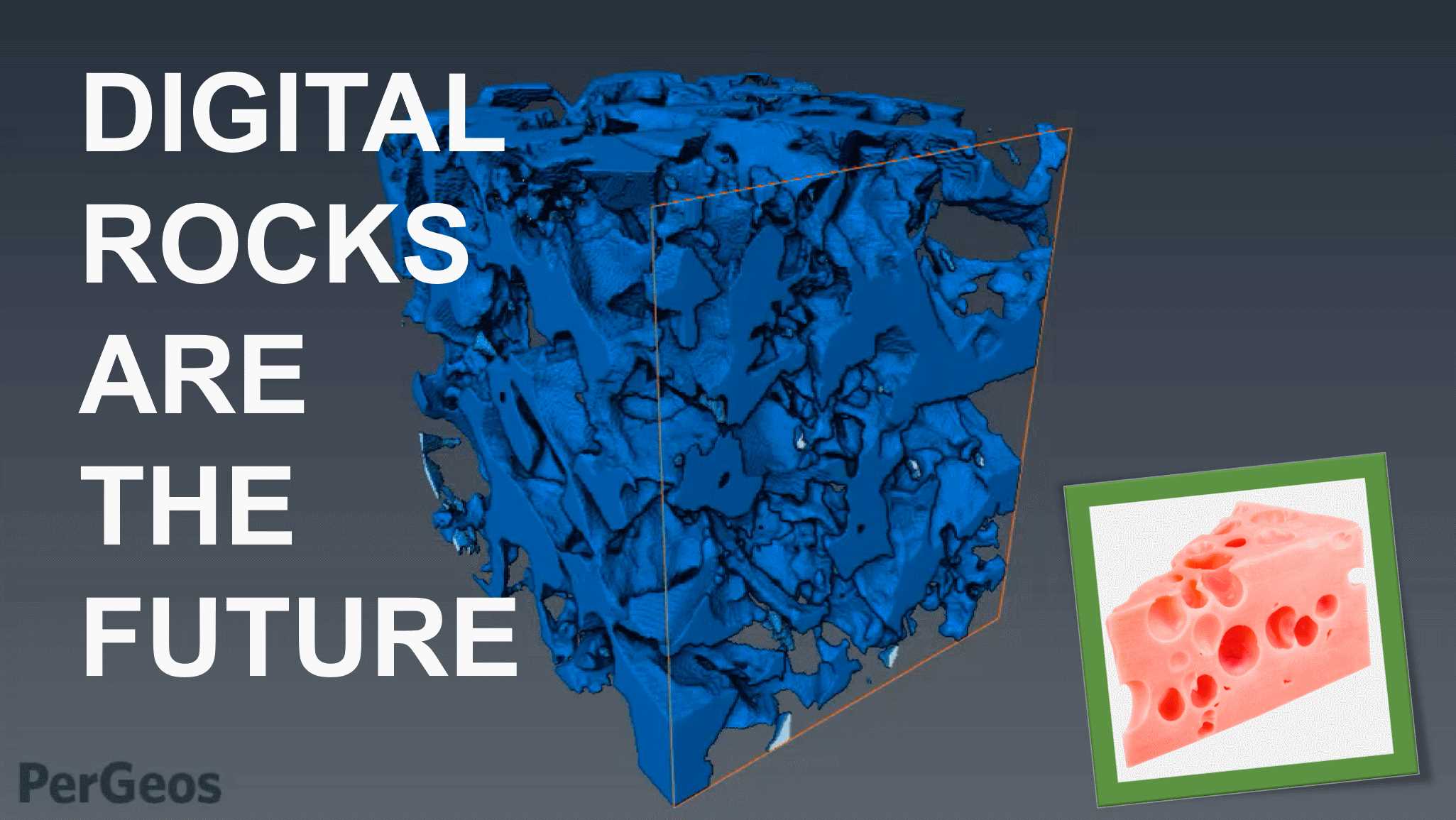
Rock analysis is not only an analog process in the laboratory anymore.

Share:          

1. Introduction
2. Step 1: Sampling
3. Step 2: Scanning -> Slice Stack
4. Step 3: Loading
5. Step 4: Noise Removal
6. Step 5: Image Segmentation
7. Step 6: Disconnected Pores
8. Step 7: Separate Unique Pores
9. Step 8: Network Model
10. Step 9: Flow Modeling
11. Videos

Introduction

The need for small-scale analysis of rocks is a common necessity in academia and industry. Digital analysis is precise and manipulation in a computer is non-destructive to the sample. This is an important consideration if the sample is rare or was expensive to obtain.

Benefits of digital analysis are the easy measurement of desired volumina and subsequent use in simulations. Digitalisation is realized with X-ray computed tomography (CT or MicroCT) or Focused Ion Beam in a Scanning Electron Microscope (FIB/SEM, which is technically destructive in a small area, since the ion beam removes layer after layer). In either case, a stack of equidistant 2d slices is created and can be used to reconstruct a 3d volume.

When sample is to be characterized it is a common task to segment and visualize and quantify pores, pore throats, post-depositional crystalizations, pore shapes etc.

I want to describe how geologists go about quantifying porosity and then model permeability from digital rocks.

Step 1: Sampling

Take a hand sample, whole core, core plug, sidewall core in the field.

Step 2: Scanning -> Slice Stack

Scan the sample with the appropriate device for the size of the sample and required resolution. The CT device will scan the sample, create a virtual model, and then export a stack of black-and-white images (so-called “slices”).

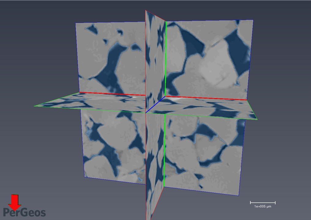
Step 3: Loading

Import stack of slices into a digital rock analysis suite. In my case, I used ThermoFisher PerGeos.

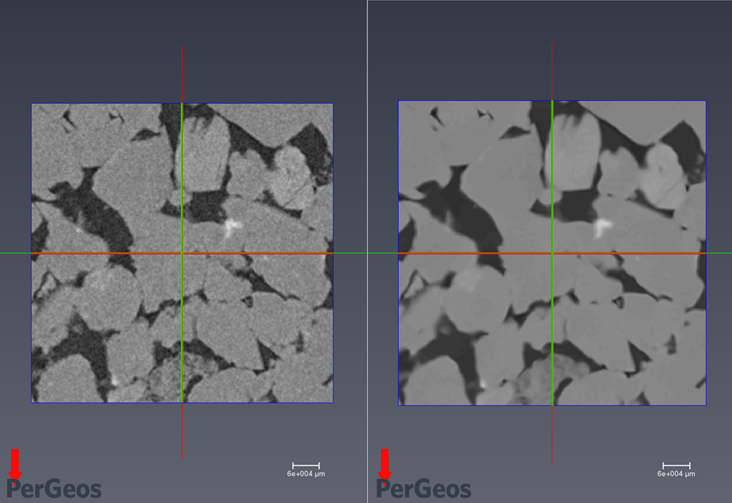
Step 4: Noise Removal

Preprocess noisy images.

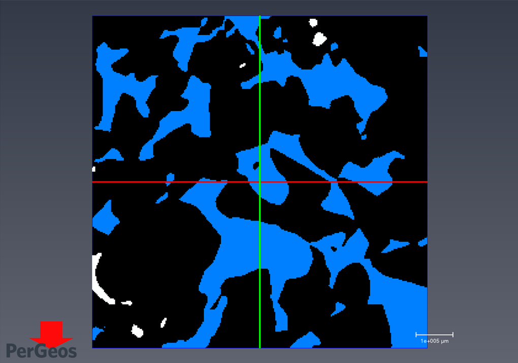
Step 5: Image Segmentation

Segment objects into classes. For example mask only the pores and assign them to class “pore space”, then mask the mineral grains etc. Various segmentation techniques exist: manual selection, magic wand, thresholding by color value, watershed. To avoid operator bias, a completely automatic routine such as wathershed should be used that delivers repeatable results.

Step 6: Disconnected Pores

Remove disconnected porosity (that has no permeability) from the total porosity and obtain the connected pore space.

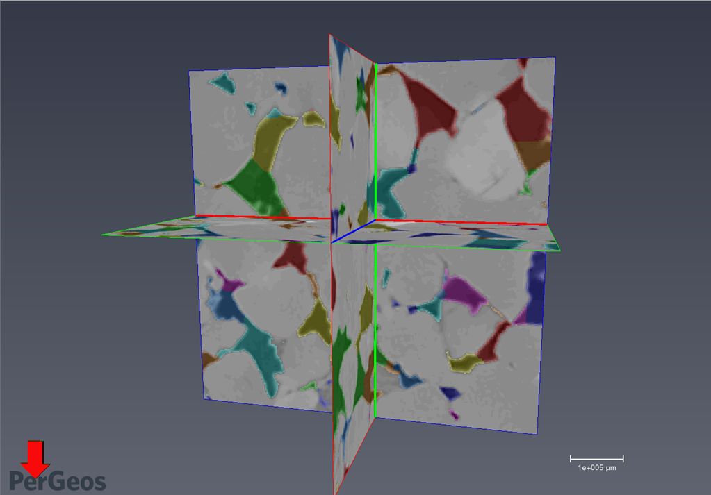
Step 7: Separate Unique Pores

Divide the total pore space into separate pores and give each an identification.

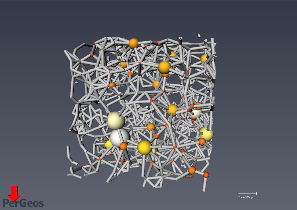
Step 8: Network Model

Generate a pore-network model.

Step 9: Flow Modeling

Model the pressure field and permeability/hydraulic conductivity (K) by setting fluid viscosity and other boundary conditions. Watch the vectorized flow pattern Single-Phase Flow Simulation through Sandstone.

Basically, this analysis pathway can also be applied to single thin sections, which were photographed under the optical microscope. In that case, no valid stack of equidistant slices is available. Some software suites can model the 3d stacking pattern of the grains if the type of rock is known. However, this is a much less quantitative approach.

The software used is ThermoFisher PerGeos 2019.4 with the freely available MicroCT dataset “Berea Sandstone Mini Plug”. More info about the Berea Sandstone and how it can be digitally processed in ThermoFisher PerGeos.

Videos

MicroCT Sandstone Porosity Segmentation

Single-Phase Flow Simulation through Sandstone