LIDAR to Digtital Elevation Models

Posted in Projectblog ∙ 7 mins read

Environmental analysis in ArcGIS

Share:          

1. Introduction
2. Step 1: Data Sourcing
3. Step 2: Loading
4. Step 3: Coordinate System
5. Step 4: Create LAS Dataset
6. Step 5: Assure geolocation
7. Step 6: Display Threshold
8. Step 8: Convert to Raster/DEM
9. Step 9: Find the right DEM Resolution
10. Step 10: Compare Multipe DEMs

Introduction

Digital Elevation Models (DEMs) are often the most basic data available about the land surface elevation and are base for many following analysis products. DEMs come in form of greyscale raster files with the elevation (Z) direction encoded in the color value. From many parts of the world these DEM datasets are already available as georeferenced raster files. However, how are they generated?

First step is recording point clouds through remote sensing techniques such as Light Detection and Ranging. The LIDAR sensor records a point where the laser is reflected from the ground together encoded elevation and spatial information. This reflection may come from a wall, a tree, water, roads, and so on. When mounted on a plane, LIDAR is a very convenient tool to get large numbers of sample points (clouds) symbolizing surface elevation.

Let’s go through the steps of creating a DEM from LIDAR point clouds.

Step 1: Data Sourcing

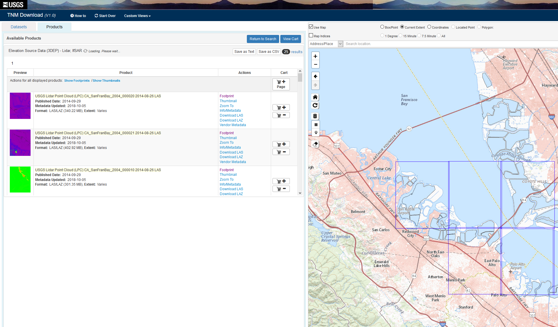
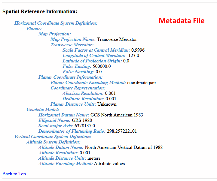
State and federal agencies of many countries provide high-quality datasets that researchers and analysts can utilize for their purposes. Online portals present the coverage of such public dataset. For example: GISgeography.com “Top 6 Free LiDAR Data Sources”. I really like The Interagency Elevation Inventory for the U.S.A. Zoom to the location in the world where you need the data from. In my example, I will use two sections from the “USGS Lidar Point Cloud (LPC) CA_SanFranBay_2004” project. The important files to download are the .LAS and the metadata (.txt or .xml).

Step 2: Loading

Many larger LIDAR projects are subdivided into sections for easier downloading. Download and unzip all the required sections to a project folder. Open ArcMap and then click on the Catalog, browse to the project folder, right click on one of the .LAS and open the file properties. Check if the provider saved the coordinate system, projection, and measurement units to the .LAS file. If the field says “Unknown”, then information has to be added manually.

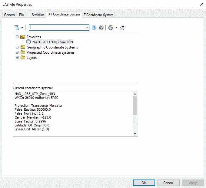
Step 3: Coordinate System

Skip this step if your coordinate system and projection are saved in the .LAS properties.

Adding the coordinate system and projection to the .LAS is not as straight forward as using the “Define Projection” tool for other features. Esri offers a separate toolbox on their website for creating a .PRJ file that contains the projection for each .LAS. Refer to this article for how to install and use the LAS Custom GP Tools for ArcGIS 10.2 toolbox that will generate .PRJ files. Make sure to follow the information given in the metadata exactly or else the point cloud may be some meters off in the best case or displayed on the other end of the world.

Step 4: Create LAS Dataset

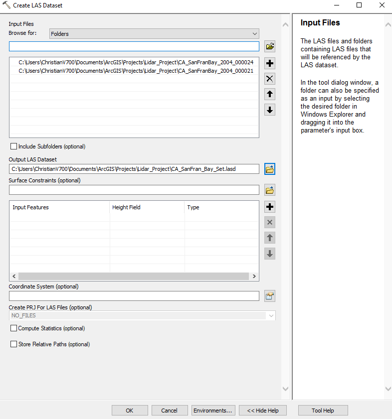
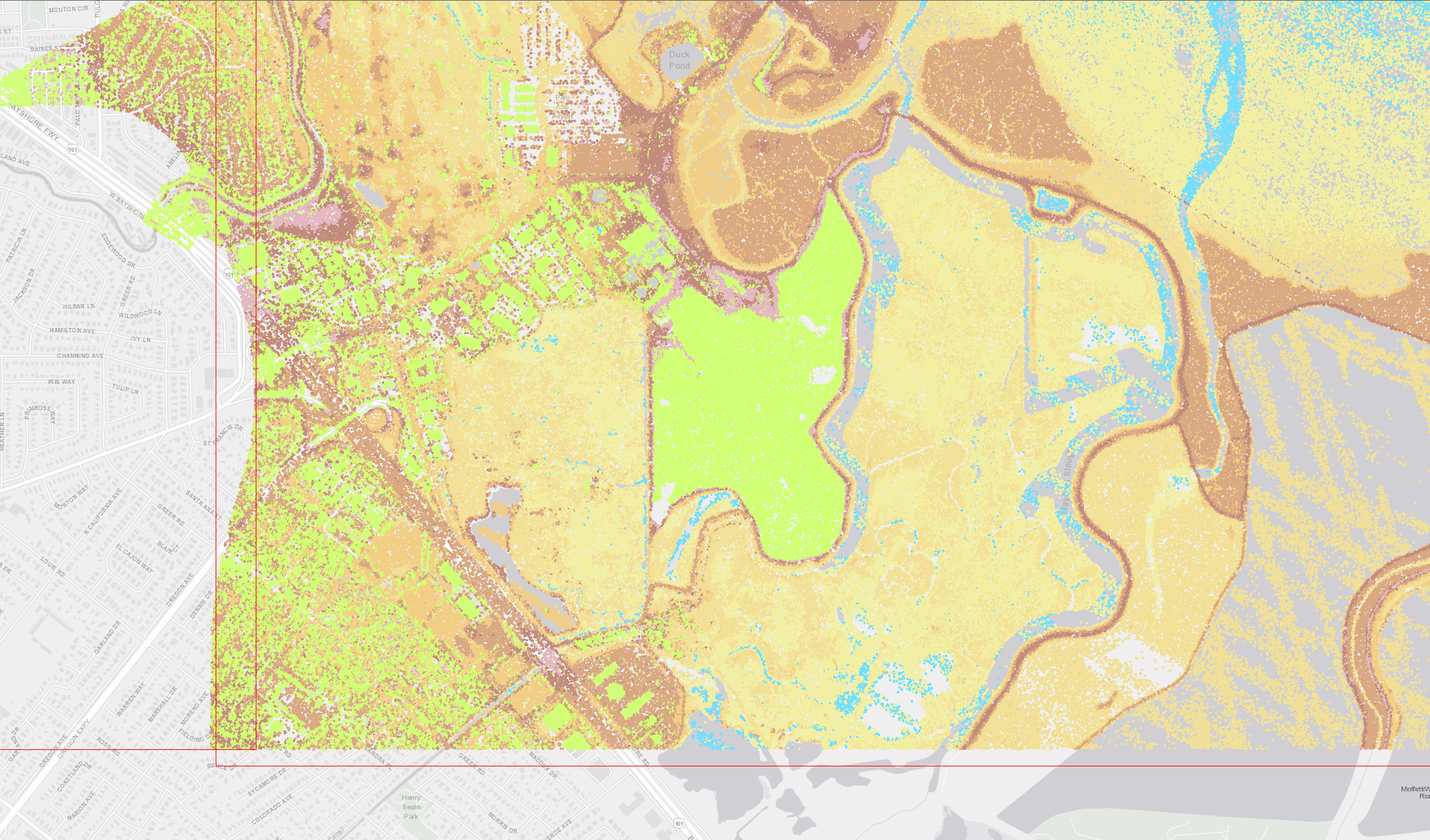
Equipped with correct .PRJ we can run tool “Create LAS Dataset”. Click “Geoprocessing” and “Search For Tools”, then enter “Create LAS Dataset”. In the “Input Files” field select all the files or folders, define an output file name with meaningful name, and activate “Store Relative Paths”. Run the tool. Then drag the new .LASD file into the Layer on the screen to display it. Red bounding boxes should show the dimensions of the LAS sections in the LAS Dataset. If no LAS points are being rendered then the zoom is too far out. My two sections combined contain a total of 82,879,066 LAS points.

Step 5: Assure geolocation

Is the point cloud where it belongs in the world? We can check by comparing with a basemap. Click “Add Data”, “Add Basemap”. Which map design is up to you. If the basemap does not show, we need to set the Layer’s projection to “WGS 1984”, which is the correct one for ArcGIS’ online basempas. The LAS Dataset will be projected on-the-fly to the WGS 1984. If everything went right, the sections will be in the same place as seen on the online portal.

Step 6: Display Threshold

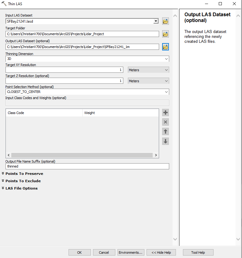
When you zoom to the layer, it may happen that nothing is going to be displayed on the map except for the red bounding frames of the .LAS dataset(s). This may be if the datasets are so detailed that ArcGiS cannot display all of them at the same time. Nothing is wrong with the data itself. First, right click the .LAS dataset in the Table of Contents and click “Properties” and then “Display”. The point limit is by defailt at 800,000. You can increase to a maximum of 5,000,000 and click “OK”. If nothing is showing, try zooming into the extent. as soon as less than five million points are on the screen, they will be displayed. You may have to do a lot of zooming and the computer will be slow. Here is another approach: my .LAS dataset contains ~83 million points. That’s huge. Use the “Thin LAS” tool to create a new downsampled point cloud. It works on both .LAS and .LASD. Define your input .LAS(D), Target Folder, and name of the new .LASD (if you use a .LASD as input). For the Target XY Resolution and Target Z Resolution enter a reasonable number such as 1 m. Run the tool and new .LAS and .LASD files will be calculated. My new dataset consists now of ~25 million points.

##Step 7: Build a TIN

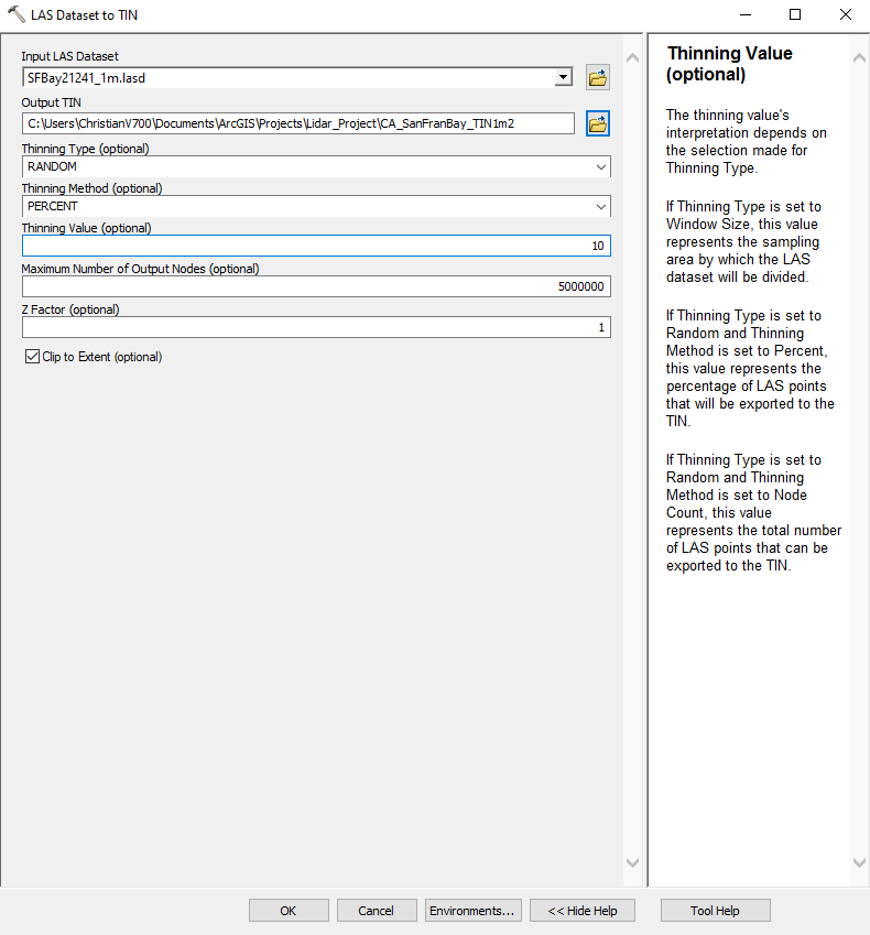
Next, we create a Triangular Irregular Network (TIN), which is a 3D surface defined by nodes connected by triangles. This is an intermediate product on the way to the DEM. This method of DEM generation is nice because it is simple to understand and does not try to do anything to fancy. Return to “Search” to find the toolbox called “LAS Dataset To TIN”. Select your .LASD in the “Input LAS Dataset” input, select your project folder and name the new file accordingly. Alternatively, if you use only a single .LAS file, use the “Create TIN” tool.

You may get the error “Too many points have been chosen to build a TIN. Either increase the amount of thinning or increase the maximum allowed output size”. In that case utilize the Thinning option, and Random Thinning Method. Try reducing the Thinning Value (in percent, 100 = no thinning) until the tool runs and creats a TIN. My new TIN was thinned to 10% and contains ~2.5 million nodes.

Step 8: Convert to Raster/DEM

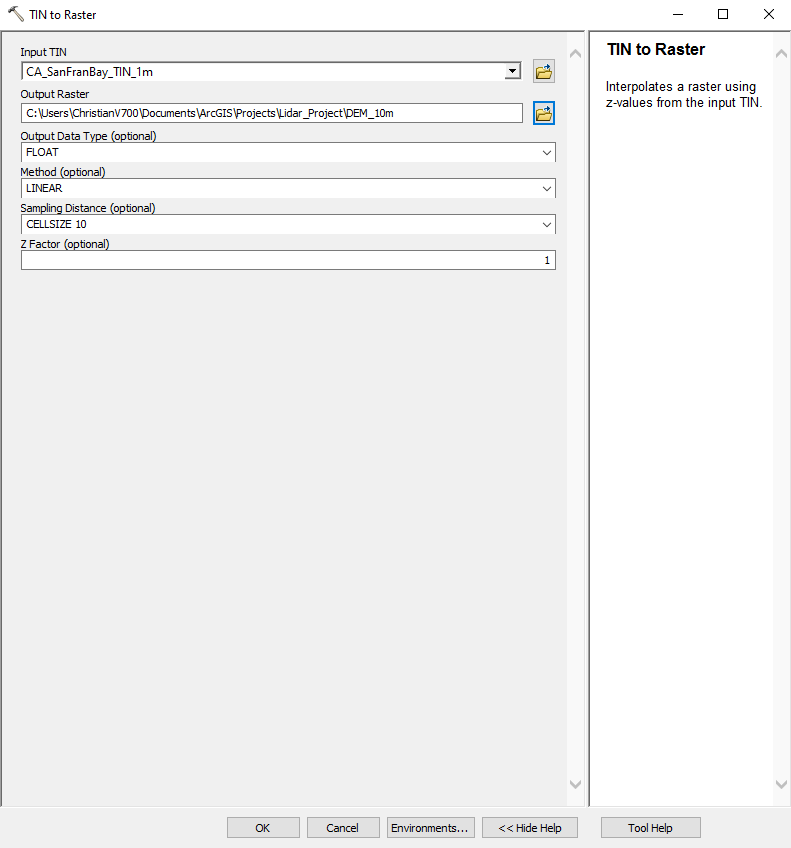
The TIN is converted to a raster, the final product. Again, return to Search and type in “TIN to Raster”. Select the TIN for input, and specify ouptut folder and name. The option “Sampling Distance” will contain precalculated values for the resolution of the DEM. Try hardcoding the cellsize (in your map unit).

Step 9: Find the right DEM Resolution

Assess the DEM. The more detailed your TIN is, the smaller you can select the cellsize (DEM resolution) without introducing artefacts. Tweak the parameters (including the Output Raster name) in order to get your desired results. You should create a set of DEMs.

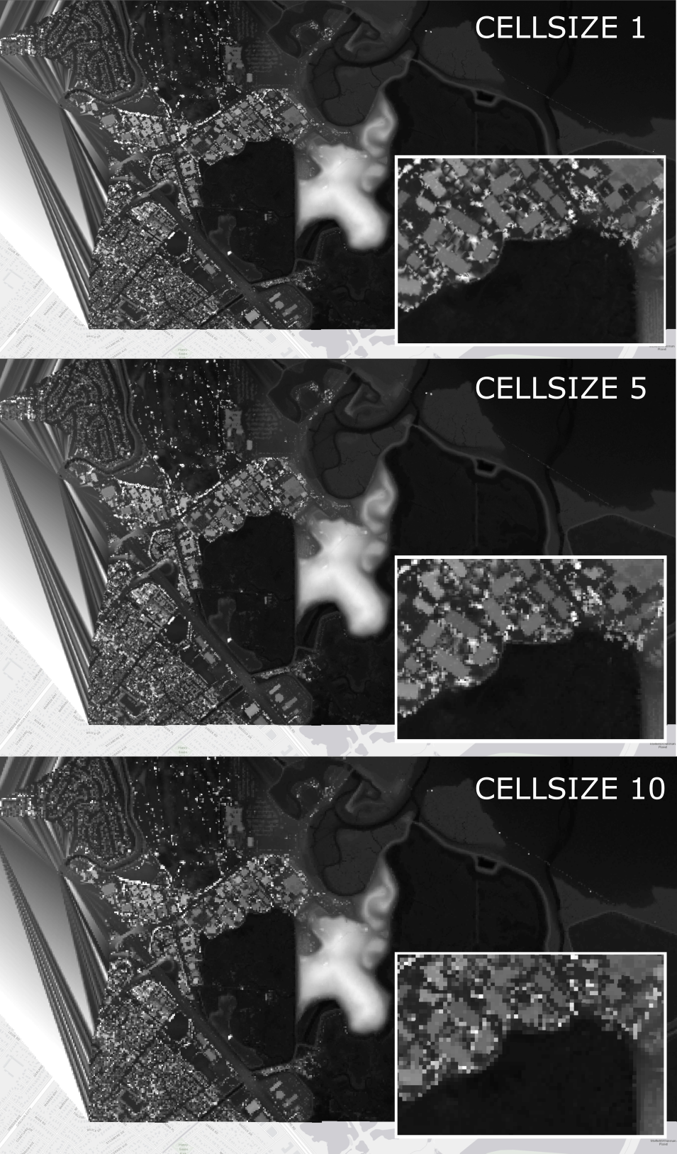
Step 10: Compare Multipe DEMs

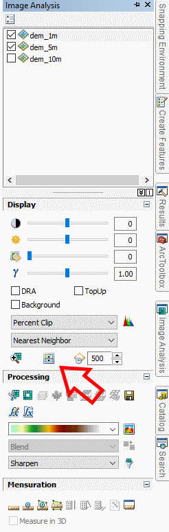
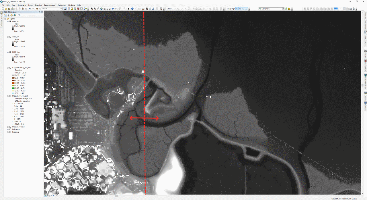
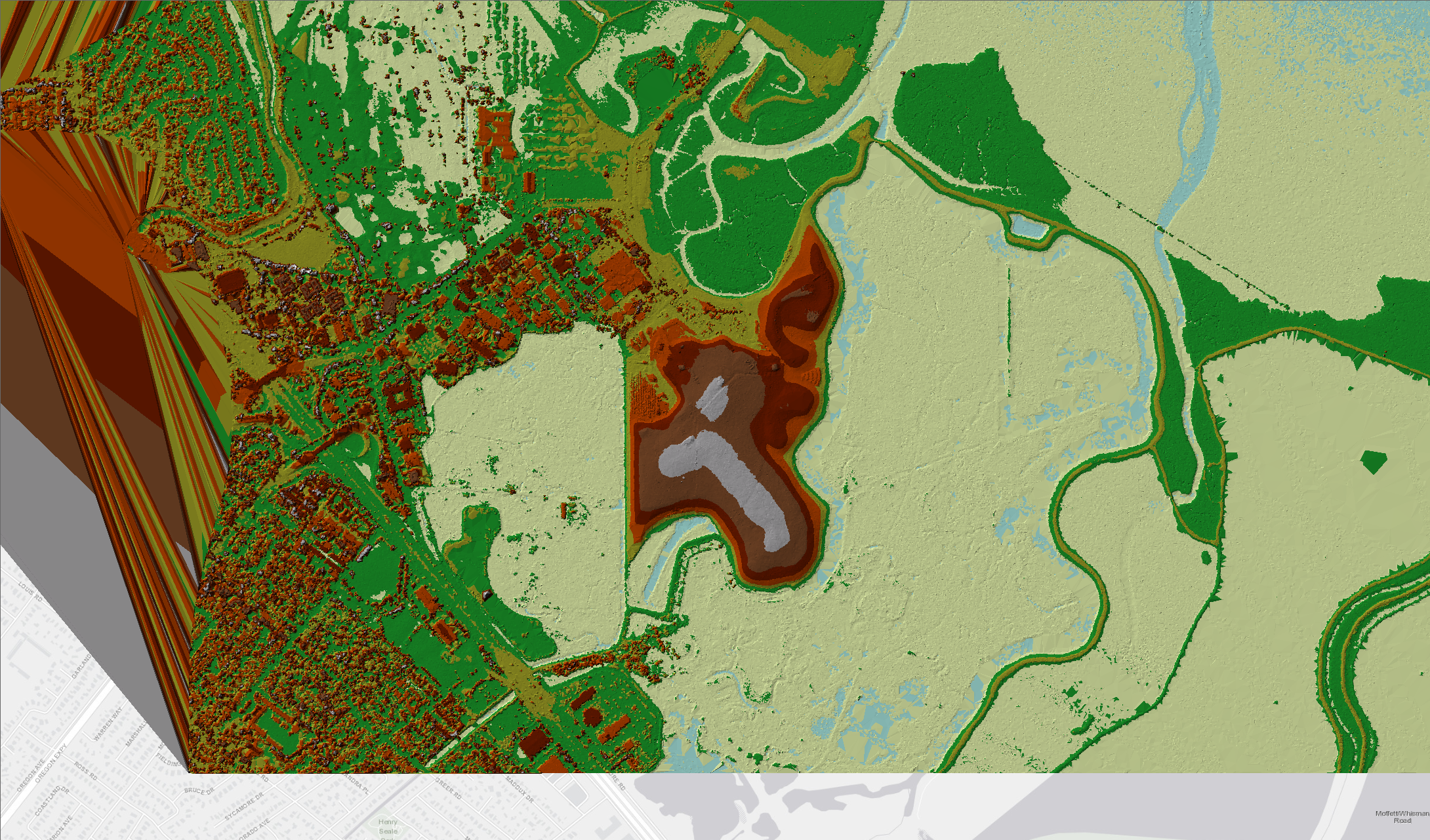
Use the Image Analysis sidebar (from the Windows menu) to compare your different DEMs. Turn on the layers for two that you would want to compare, and use the Slider Tool (red arrow) to drag across the images and compare them. For the final product select the DEM with smallest cellsize and minimal artefacts. Note that the 1m-DEM contains many artefacts especially visible near the houses, which was introduced by reducing the TIN size down from the 1m LAS dataset. The 5m DEM is a better compromise.