Landsat Imagery Classification

Posted in Projectblog ∙ 5 mins read

Quantify the Burned Forest Area in Australia

Share:          

1. Introduction
2. Analysis
3. Results
4. Conclusions

Introduction

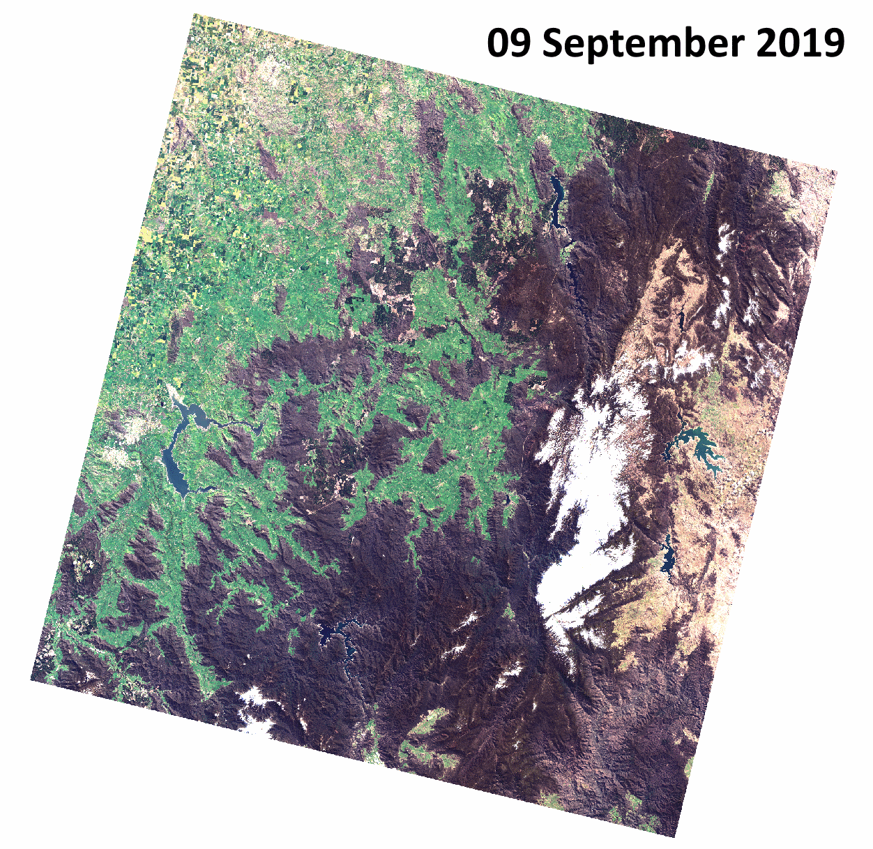
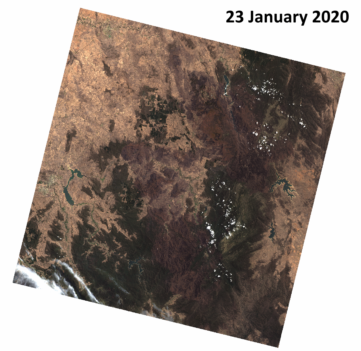
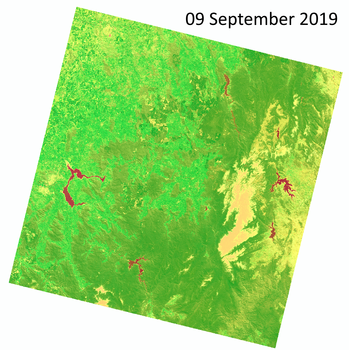
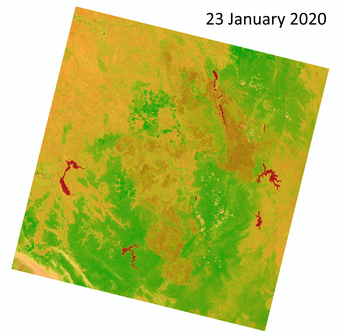
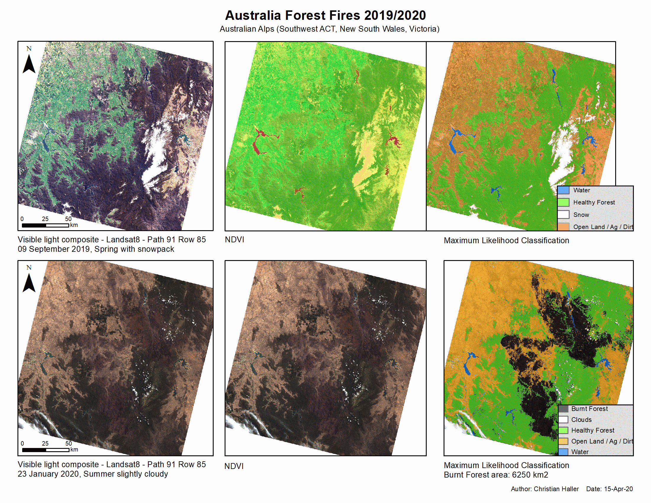
Fires ravaged the forested south of Australia in the past dry season and made global headlines in January 2020. I chose to compare Landsat imagery of the Australian Alps from last Spring and Summer, i.e. pre and post fire to assess the area of burnt forest. The selected tile Path 91 Row 85 covers the southwestern corner of the Australian Capital Territory (ACT) and the New South Wales/Victoria territory border. To achieve such an analysis, ca. 10 time slices of Landsat 8 imagery were requested from USGS EarthExplorer covering September 2019 and April 2020. Many slices were discarded due to high cloud coverage, smoke, and haze that would make classification ambiguous. Selected time slices were 09 September 2019 (Spring / pre-burn) and 23 January 2020 (Summer / post-burn).

In the following I show how to train a classification model that quantifies the burnt area. The nexts steps will have to be completed twice, once for each seasonal image.

Analysis

Step 1

Unpack the Landsat8 files and use the tool “Composite Bands” in ArcGIS that combines multiple wavelength band images into a single image. Landsat8’s band assignment can be taken from the metadata in each compressed file. Red = Band 4, Green = Band 3, Blue = Band 2.

Step 2

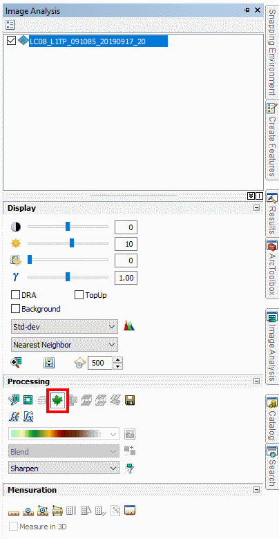
Create an NDVI raster. NDVI is an acronym for Normalized Difference Vegetation Index and uses the Red and the Near Infrared bands NDVI = (NIR - Red)/(NIR + Red). Higher values of the index indicate light reflected by vegetation, low values indicate the absence of vegetation. We could use the Raster Calculator, but ArcGIS has an integrated feature for quck and reliable creaton of such a raster. Activate the “Image Analysis” from the “Windows” menue. Click on the little leaf icon. Assess the image and if you want, change the color ramp. For example from red to green and add some transparency.

The burn scars in the mountains should be visible as broad areas of low NDVI, ranging from northwest to southeast.

Step 3

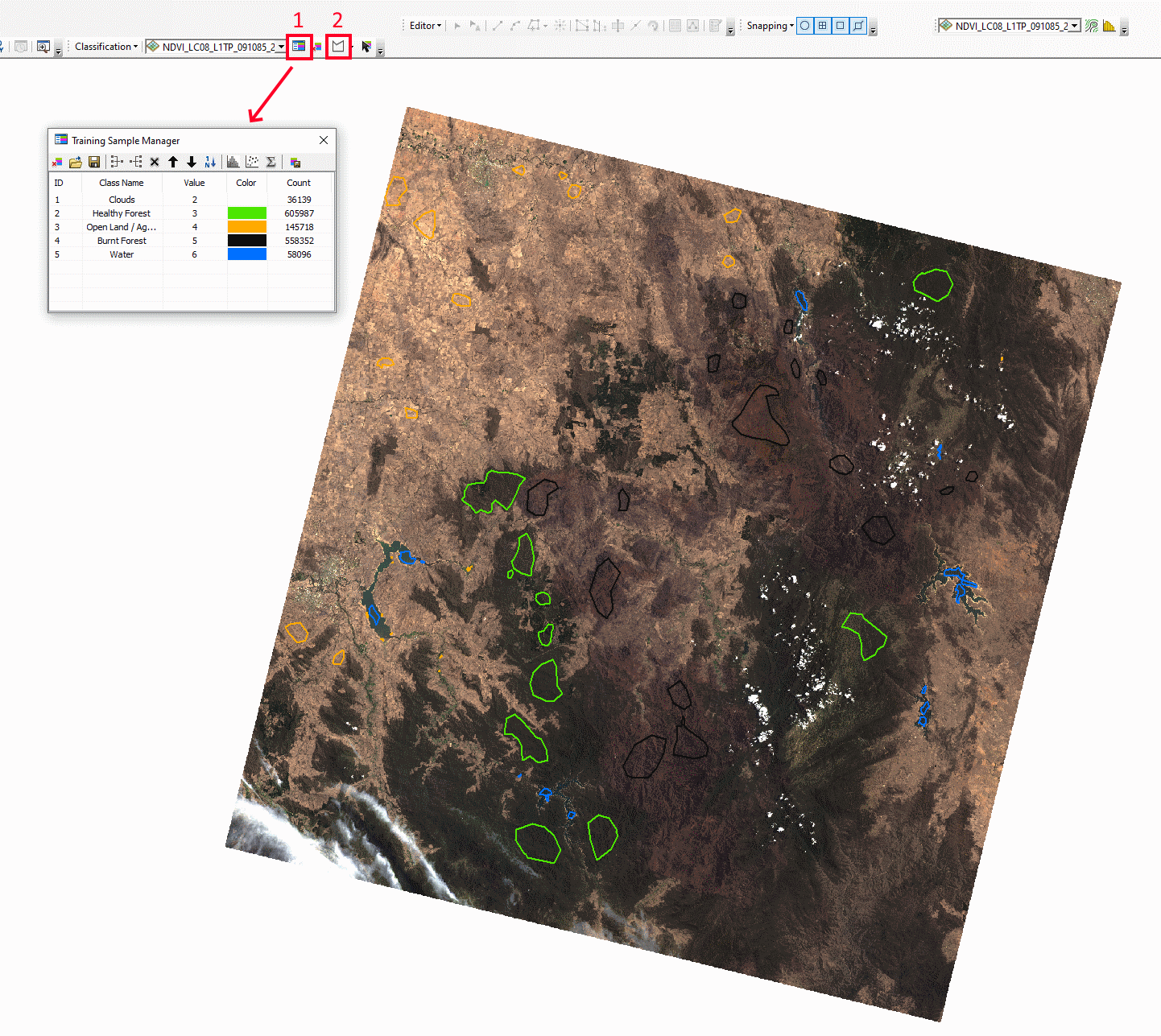
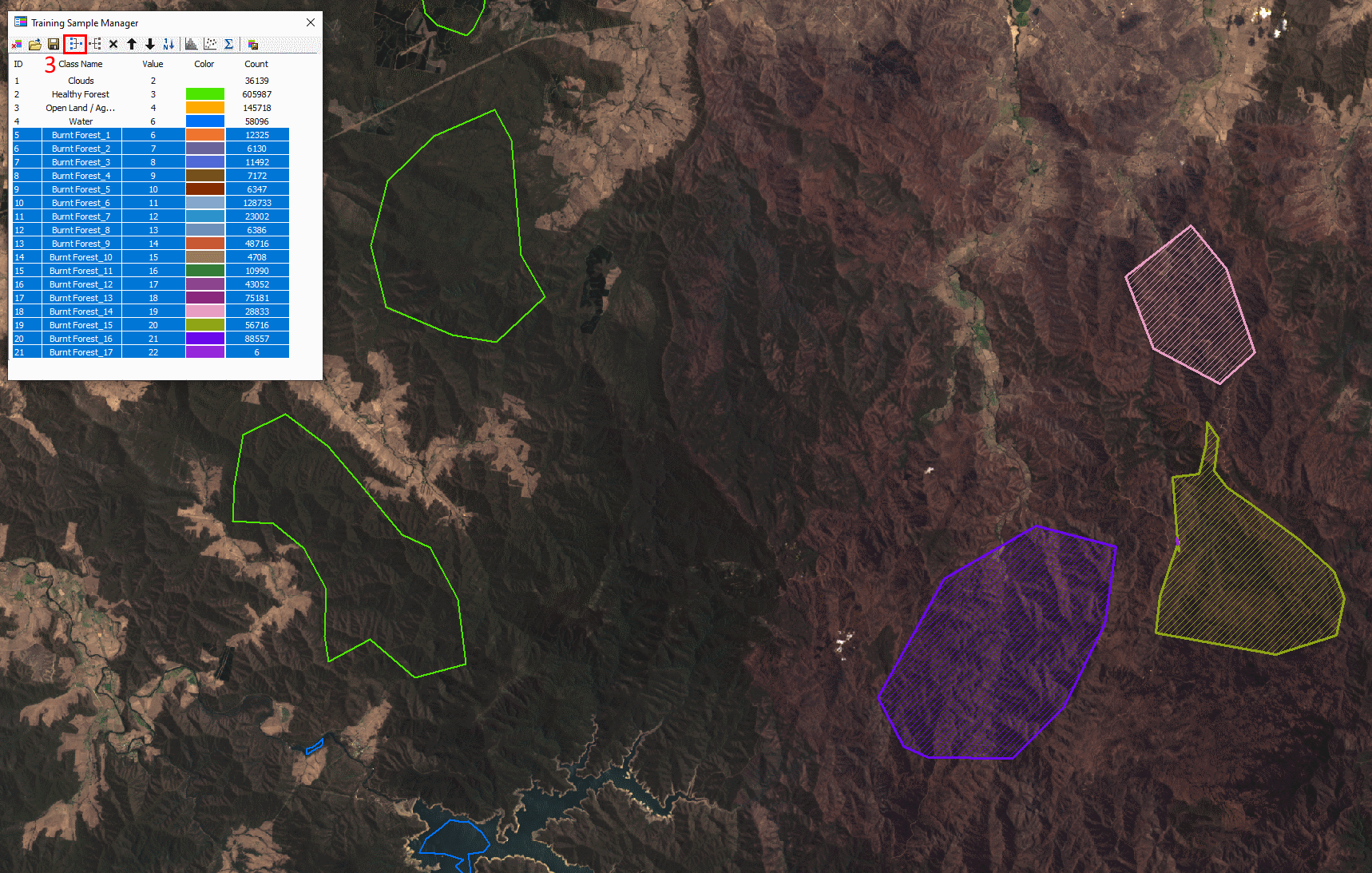
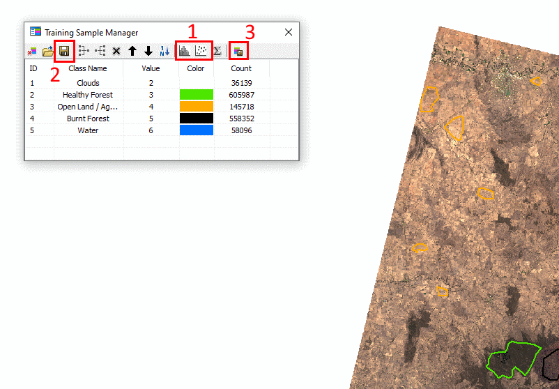
Enable the “Image Classification” Toolbar. On the Image Classification Toolbar click on the Sample Manager (1). Here you can add polygons that represent color values of your classes (2) by clicking into the raster image. Add a minimum of 10 samples for each class you want to record to cover as much variability across the image as possible. In the forest fire case we should take samples of “Water” (lakes, rivers), “Open Land” (dirt, grassland etc.), “Healthy Forest”, “Burnt Forest” and if applicable “Snow” or “Clouds”. I suggest you do not classify towns and other human infrastructure, since it is harder to distinguish from other classes and beyond the scope of this project. When you are done, click “Merge Training Samples” (3), rename the class name, and select an intuitive color. The training samples of your first classification can potentially be reused in the second classification by clicking the “Load Training Samples” button, but make sure all classes are still well represented and make adjustments when necessary.

Step 4

Next step is the assessment the samples. Ideally, all classes are well separated and do not have overlapping colors. Click on the Histogram and Scatterplot icons (1) and judge how much overlap exists. When you are satisfied with your work, save the classification shapes (2) and then train the model by clicking on “Create a Signature File” (3).

Step 5

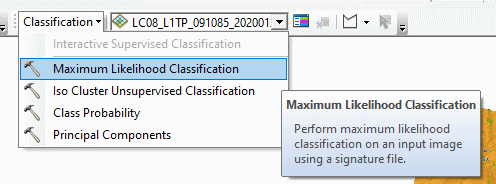
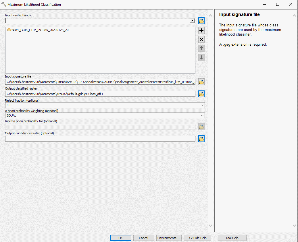
Using the signature file we can make predictions for the entire image in a classification raster. In the “Image Classification Toolbar” click “Classification”, in the menue then select the “Maximum Likelihood Classification” Tool. This new raster contains the count of cells for each class, but not the real area we want.

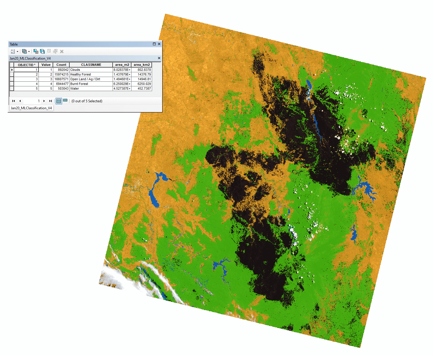
So either add a field to the Attribute Table and use the “Field Calculator” (Landsat8 cells are 30 m edge length = 900 m² per cell) or convert the classification raster to a feature, which pre-calculates the area values (“Raster to Polygon” tool, tick “multipart features”).

Results

No Burnt Forests were visible in September 2019’s NDVI, hence no training shapes were used for classifying Burnt Forests and it has to be assumed 0 km² were charred.

A total of 6250 km² were measured in January 2020 few days to weeks after the forest fires in the selected Landsat8 imagery.

Conclusions

The burnt forest areas of southeast Australia are reliably located using NDVI and quantified using the Maximum Likelihood Classification tool, which is a proof-of-concept.

Future research may include:

• Assessment of recovery of the burnt forests, which includes timing the return of normal NDVI values and spatial progress plant colonization.
• Quantifying the severity of burns using the Normalized Burn Ratio which uses the the Near Infrared and Shortwave Infrared bands in the following formula NBR = (NIR - SWIR) / (NIR + SWIR). This proof-of-concept study confirms that classification can be feasible and automated using the Model Builder.
• Automation of new time slices with the ModelBuilder of processing except for initial quality assessment of the image (cloudiness and color distortion?) and Training Sample selection