Cats vs. Dogs in TensorFlow Part I
Cats Vs. Dogs computer vision with the TensorFlow API
- Introduction
- Step 1: Explore the Example Data of Cats and Dogs
- Step 2: Build a Convolutional Neural Network
- Step 3: Pre-Processing - Image Data Generator
- Step 4: Training
- Step 5: Visualizing Intermediate Representations (Optional)
- Step 6: Making predictions
- Step 7: Evaluate the Training and Validation accuracy
- Acknowledgements:
Introduction
In a previous post about computer vision I wrote how to make binary predictions if a photo contains a cat or no cat Article “Cat Prediction”. This was a much simpler classifier built from ground up. However, not many users would still programm everything from scratch today. It is much easier to make use of a Deep Learning API such as PyTorch, Keras, TensorFlow etc.
For this project, we will take that to the next level, recognizing real images of Cats and Dogs in order to classify an incoming image as one or the other using Google’s TensorFlow. This API has many functions already built in so that they only have to be called with a single line of code or even set only a parameter.
For example, as part of the task we need to process the data - not least resizing it to be uniform in shape.
We will follow these steps:
- Explore the Example Data of Cats and Dogs
- Build a Convolutional Neural Network
- Data Preprocessing
- Training
- Visualizing Intermediate Representations (Optional)
- Making predictions
- Evaluate the Training and Validation accuracy
If you want to follow along on the Jupyter notebook hosted on GitHub click on this link, otherwise keep on reading.
Step 1: Explore the Example Data of Cats and Dogs
Let’s start by downloading our example data, a .zip of 2,000 JPG pictures of cats and dogs, and extracting it locally in \Data . Note: The place where your Jupyter file is stored is the working directory.
The 2,000 images used in this exercise are excerpted from the “Dogs vs. Cats” dataset available on Kaggle, which contains 25,000 images. Here, we use a subset of the full dataset to decrease training time for practial purposes.
import os
import wget

url = 'https://storage.googleapis.com/mledu-datasets/cats_and_dogs_filtered.zip'
wget.download(url, out=f'{os.getcwd()}\\Data\\cats_and_dogs_filtered.zip')
The following code will use the OS library to use Operating System libraries, giving you access to the working directory, and the zipfile library allowing you to unzip the data.
import zipfile

local_zip = f'{os.getcwd()}\\Data\\cats_and_dogs_filtered.zip'

zip_ref = zipfile.ZipFile(local_zip, 'r')

zip_ref.extractall(f'{os.getcwd()}\\Data')
zip_ref.close()
The contents of the .zip are extracted to the base directory \Data\cats_and_dogs_filtered, which contains train and validation subdirectories for the training and validation datasets, which in turn each contain cats and dogs subdirectories.
In Summary: The Training Set are the photos that are used to tell the model that this is what cats and dogs look like. The Validation Set contains images of cats and dogs that the model will not see as part of the training, so we can test how it does in evaluating if an image contains a cat or a dog.
The practical thing about TensorFlow: We do not explicitly label the images as cats or dogs. We will use the ImageGenerator, which is used to read images from subdirectories, and automatically label the data contained with the name of that subdirectory. So we will have a ‘Training’ directory containing a ‘Cats’ directory and a ‘Dogs’ one. The ImageGenerator will label the images appropriately for us and saving us time.
First we have to define the paths to all these directories:
base_dir = f'{os.getcwd()}\\Data\\cats_and_dogs_filtered'

train_dir = os.path.join(base_dir, 'train')
validation_dir = os.path.join(base_dir, 'validation')

# Directory with our training cat/dog pictures
train_cats_dir = os.path.join(train_dir, 'cats')
train_dogs_dir = os.path.join(train_dir, 'dogs')

# Directory with our validation cat/dog pictures
validation_cats_dir = os.path.join(validation_dir, 'cats')
validation_dogs_dir = os.path.join(validation_dir, 'dogs')
Now, let’s see what the file names look like in the cats and dogs train directories (file naming conventions are the same in the validation directory):
train_cat_fnames = os.listdir( train_cats_dir )
train_dog_fnames = os.listdir( train_dogs_dir )

print(train_cat_fnames[:10])
print(train_dog_fnames[:10])
Result:
['cat.0.jpg', 'cat.1.jpg', 'cat.10.jpg', 'cat.100.jpg', 'cat.101.jpg', 'cat.102.jpg', 'cat.103.jpg', 'cat.104.jpg', 'cat.105.jpg', 'cat.106.jpg']
['dog.0.jpg', 'dog.1.jpg', 'dog.10.jpg', 'dog.100.jpg', 'dog.101.jpg', 'dog.102.jpg', 'dog.103.jpg', 'dog.104.jpg', 'dog.105.jpg', 'dog.106.jpg']
Let’s find out the total number of cat and dog images in the train and validation directories:
print('total training cat images :', len(os.listdir(      train_cats_dir ) ))
print('total training dog images :', len(os.listdir(      train_dogs_dir ) ))

print('total validation cat images :', len(os.listdir( validation_cats_dir ) ))
print('total validation dog images :', len(os.listdir( validation_dogs_dir ) ))
Result:
total training cat images : 1000
total training dog images : 1000
total validation cat images : 500
total validation dog images : 500
For both cats and dogs, we have 1,000 training images and 500 validation images.
Now let’s take a look at a few pictures to get a better sense of what the cat and dog datasets look like. First, configure the matplot parameters:
%matplotlib inline

import matplotlib.image as mpimg
import matplotlib.pyplot as plt

# Parameters for our graph; we'll output images in a 4x4 configuration
nrows = 4
ncols = 4

pic_index = 0 # Index for iterating over images
Now, display a batch of eight cat and eight dog pictures. Each time this code is called, a new set of pictures will appear.
# Set up matplotlib fig, and size it to fit 4x4 pics

fig = plt.gcf()
fig.set_size_inches(ncols*4, nrows*4)

pic_index+=8

next_cat_pix = [os.path.join(train_cats_dir, fname)
                for fname in train_cat_fnames[ pic_index-8:pic_index]
               ]

next_dog_pix = [os.path.join(train_dogs_dir, fname)
                for fname in train_dog_fnames[ pic_index-8:pic_index]
               ]

for i, img_path in enumerate(next_cat_pix+next_dog_pix):
  # Set up subplot; subplot indices start at 1
  sp = plt.subplot(nrows, ncols, i + 1)
  sp.axis('Off') # Don't show axes (or gridlines)

  img = mpimg.imread(img_path)
  plt.imshow(img)

plt.show()
Result:
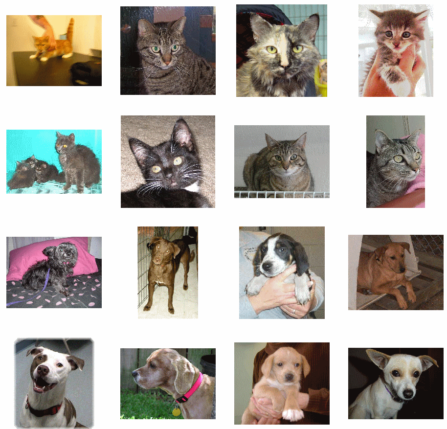
The images are in color and come in a variety of shapes. Before training a Neural network with them we will need to tweak the images. We will see that in the next section.
Ok, now that you have an idea for what your data looks like, the next step is to define the model that will be trained to recognize cats or dogs from these images.
Step 2: Build a Convolutional Neural Network
First of all, we need to import TensorFlow and best check for the installed version.
This simple neural network will start with images of the size 150 x 150 pixels and three color values (RGB). It will contain three convolutional layers followed by pooling layers, which reduce the number of pixels. Then the 2D images will be flattened out to a single row of pixels that become neurons. After that, a fully connected layer (dense) with ReLu and then already the output layer with a single neuron that will indicate 1 or 0 for cat or dog. Activation for that final neuron will be a sigmoid function.
import tensorflow as tf
print("TensorFlow version: ",tf.__version__)

model = tf.keras.models.Sequential([
	# Note the input shape is the desired size of the image 150x150 with 3 bytes color
	tf.keras.layers.Conv2D(16, (3,3), activation='relu', input_shape=(150, 150, 3)),
	tf.keras.layers.MaxPooling2D(2,2),

	tf.keras.layers.Conv2D(32, (3,3), activation='relu'),
	tf.keras.layers.MaxPooling2D(2,2),

	tf.keras.layers.Conv2D(64, (3,3), activation='relu'),
	tf.keras.layers.MaxPooling2D(2,2),

	# Flatten the results to feed into a DNN
	tf.keras.layers.Flatten(),

	# 512 neuron hidden layer
	tf.keras.layers.Dense(512, activation='relu'),

	# Only 1 output neuron. It will contain a value from 0-1 where 0 for 1 class ('cats') and 1 for the other ('dogs')
	tf.keras.layers.Dense(1, activation='sigmoid')
	])
The model layout can be shown by calling the summary method.
model.summary()
Result:
Model: "sequential"
_________________________________________________________________
Layer (type)                 Output Shape              Param #
=================================================================
conv2d (Conv2D)              (None, 148, 148, 16)      448
_________________________________________________________________
max_pooling2d (MaxPooling2D) (None, 74, 74, 16)        0
_________________________________________________________________
conv2d_1 (Conv2D)            (None, 72, 72, 32)        4640
_________________________________________________________________
max_pooling2d_1 (MaxPooling2 (None, 36, 36, 32)        0
_________________________________________________________________
conv2d_2 (Conv2D)            (None, 34, 34, 64)        18496
_________________________________________________________________
max_pooling2d_2 (MaxPooling2 (None, 17, 17, 64)        0
_________________________________________________________________
flatten (Flatten)            (None, 18496)             0
_________________________________________________________________
dense (Dense)                (None, 512)               9470464
_________________________________________________________________
dense_1 (Dense)              (None, 1)                 513
=================================================================
Total params: 9,494,561
Trainable params: 9,494,561
Non-trainable params: 0
__________________________
The “output shape” column shows how the size of the feature map evolves in each successive layer. The convolution layers reduce the size of the feature maps by a bit due to lack of padding, and each pooling layer halves the dimensions.
Next, we will set more model configurations. We will train the model with the binary_crossentropy loss, because it is a binary classification problem (cat,dog) and our final activation is a sigmoid. We will use the rmsprop optimizer with a learning rate of 0.001. During training, we will want to monitor classification “accuracy”.
from tensorflow.keras.optimizers import RMSprop

model.compile(optimizer=RMSprop(lr=0.001),
              loss='binary_crossentropy',
              metrics = ['accuracy'])
Step 3: Pre-Processing - Image Data Generator
Let’s configure the data generators that will read pictures in our source folders, convert them to float32 tensors, and feed them including labels to the neural network. Training images and validation images will be separate generators. The generators will yield batches of 20 images of size 150x150 and their labels (binary).
Statistical modeling data should usually be normalized to make it more amenable to processing by the network. In our case, we will preprocess our images by normalizing the pixel values to be in the 0 to 1 range. Originally all values are in the 0 to 255 range.
In Keras this can be done via the keras.preprocessing.image.ImageDataGenerator class using the rescale parameter. This ImageDataGenerator class allows you to instantiate generators of augmented image batches (and their labels) via .flow(data, labels) or .flow_from_directory(directory). These generators can then be used with the Keras model methods that accept data generators as inputs: fit, evaluate_generator, and predict_generator.
from tensorflow.keras.preprocessing.image import ImageDataGenerator

# All images will be rescaled by 1./255.
train_datagen = ImageDataGenerator( rescale = 1.0/255. )
test_datagen  = ImageDataGenerator( rescale = 1.0/255. )

# --------------------
# Flow training images in batches of 20 using train_datagen generator
# --------------------
train_generator = train_datagen.flow_from_directory(train_dir,
                                                    batch_size=20,
                                                    class_mode='binary',
                                                    target_size=(150, 150))
# --------------------
# Flow validation images in batches of 20 using test_datagen generator
# --------------------
validation_generator =  test_datagen.flow_from_directory(validation_dir,
                                                         batch_size=20,
                                                         class_mode  = 'binary',
                                                         target_size = (150, 150))
Step 4: Training
Let’s train on all 2,000 images available, for 15 epochs, and validate on all 1,000 test images.
TensorFlow will print four metrics per epoch – Loss, Accuracy, Validation Loss and Validation Accuracy.
The Loss and Accuracy are a great indication of progress of Training. It’s making a guess as to the classification of the training data, and then measuring it against the known label, calculating the result. Accuracy is the portion of correct guesses.
The Validation Accuracy is the measurement with the data that has not been used in training. As expected this would be a bit lower.
history = model.fit(train_generator,
					validation_data=validation_generator,
					steps_per_epoch=100,
					epochs=15,
					validation_steps=50,
					verbose=2)
Result:
Epoch 1/15
100/100 - 17s - loss: 0.7927 - accuracy: 0.5525 - val_loss: 0.6704 - val_accuracy: 0.6120
Epoch 2/15
100/100 - 7s - loss: 0.6163 - accuracy: 0.6635 - val_loss: 0.6668 - val_accuracy: 0.6150
Epoch 3/15
100/100 - 7s - loss: 0.5260 - accuracy: 0.7415 - val_loss: 0.5673 - val_accuracy: 0.7150
Epoch 4/15
100/100 - 7s - loss: 0.4682 - accuracy: 0.7745 - val_loss: 0.5919 - val_accuracy: 0.7070
Epoch 5/15
100/100 - 7s - loss: 0.3799 - accuracy: 0.8245 - val_loss: 0.5949 - val_accuracy: 0.7080
Epoch 6/15
100/100 - 7s - loss: 0.2923 - accuracy: 0.8705 - val_loss: 0.6991 - val_accuracy: 0.7180
Epoch 7/15
100/100 - 7s - loss: 0.2027 - accuracy: 0.9250 - val_loss: 0.8081 - val_accuracy: 0.7170
Epoch 8/15
100/100 - 7s - loss: 0.1384 - accuracy: 0.9460 - val_loss: 1.1282 - val_accuracy: 0.6960
Epoch 9/15
100/100 - 7s - loss: 0.1163 - accuracy: 0.9585 - val_loss: 1.0216 - val_accuracy: 0.7030
Epoch 10/15
100/100 - 7s - loss: 0.0761 - accuracy: 0.9735 - val_loss: 1.4962 - val_accuracy: 0.7060
Epoch 11/15
100/100 - 8s - loss: 0.0565 - accuracy: 0.9825 - val_loss: 1.3429 - val_accuracy: 0.7210
Epoch 12/15
100/100 - 7s - loss: 0.0486 - accuracy: 0.9835 - val_loss: 1.5935 - val_accuracy: 0.7040
Epoch 13/15
100/100 - 7s - loss: 0.0420 - accuracy: 0.9850 - val_loss: 1.4677 - val_accuracy: 0.7290
Epoch 14/15
100/100 - 7s - loss: 0.0469 - accuracy: 0.9855 - val_loss: 1.7934 - val_accuracy: 0.7110
Epoch 15/15
100/100 - 7s - loss: 0.0430 - accuracy: 0.9890 - val_loss: 2.0219 - val_accuracy: 0.7080
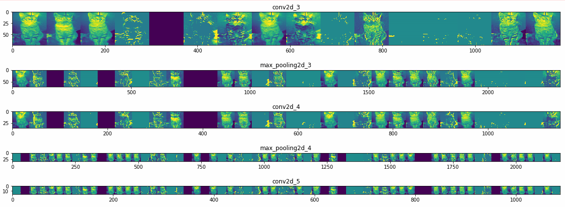
Step 5: Visualizing Intermediate Representations (Optional)
To get a feel for what kind of features the convolutional network has learned, one fun thing to do is to visualize how an input gets transformed as it goes through the network.
Let’s pick a random cat or dog image from the training set, and then generate a figure where each row is the output of a layer, and each image in the row is a specific filter in that output feature map. Rerun this cell to generate intermediate representations for a variety of training images.
import numpy as np
import random
from   tensorflow.keras.preprocessing.image import img_to_array, load_img

# Let's define a new Model that will take an image as input, and will output
# intermediate representations for all layers in the previous model after
# the first.
successive_outputs = [layer.output for layer in model.layers[1:]]

#visualization_model = Model(img_input, successive_outputs)
visualization_model = tf.keras.models.Model(inputs = model.input, outputs = successive_outputs)

# Let's prepare a random input image of a cat or dog from the training set.
cat_img_files = [os.path.join(train_cats_dir, f) for f in train_cat_fnames]
dog_img_files = [os.path.join(train_dogs_dir, f) for f in train_dog_fnames]

img_path = random.choice(cat_img_files + dog_img_files)
img = load_img(img_path, target_size=(150, 150))  # this is a PIL image

x   = img_to_array(img)                           # Numpy array with shape (150, 150, 3)
x   = x.reshape((1,) + x.shape)                   # Numpy array with shape (1, 150, 150, 3)

# Rescale by 1/255
x /= 255.0

# Let's run our image through our network, thus obtaining all
# intermediate representations for this image.
successive_feature_maps = visualization_model.predict(x)

# These are the names of the layers, so can have them as part of our plot
layer_names = [layer.name for layer in model.layers]

# -----------------------------------------------------------------------
# Now let's display our representations
# -----------------------------------------------------------------------
for layer_name, feature_map in zip(layer_names, successive_feature_maps):

  if len(feature_map.shape) == 4:

    #-------------------------------------------
    # Just do this for the conv / maxpool layers, not the fully-connected layers
    #-------------------------------------------
    n_features = feature_map.shape[-1]  # number of features in the feature map
    size       = feature_map.shape[ 1]  # feature map shape (1, size, size, n_features)

    # We will tile our images in this matrix
    display_grid = np.zeros((size, size * n_features))

    #-------------------------------------------------
    # Postprocess the feature to be visually palatable
    #-------------------------------------------------
    for i in range(n_features):
      x  = feature_map[0, :, :, i]
      x -= x.mean()
      x /= x.std ()
      x *=  64
      x += 128
      x  = np.clip(x, 0, 255).astype('uint8')
      display_grid[:, i * size : (i + 1) * size] = x # Tile each filter into a horizontal grid

    #-----------------
    # Display the grid
    #-----------------

    scale = 20. / n_features
    plt.figure( figsize=(scale * n_features, scale) )
    plt.title ( layer_name )
    plt.grid  ( False )
    plt.imshow( display_grid, aspect='auto', cmap='viridis' )
Result:
Step 6: Making predictions
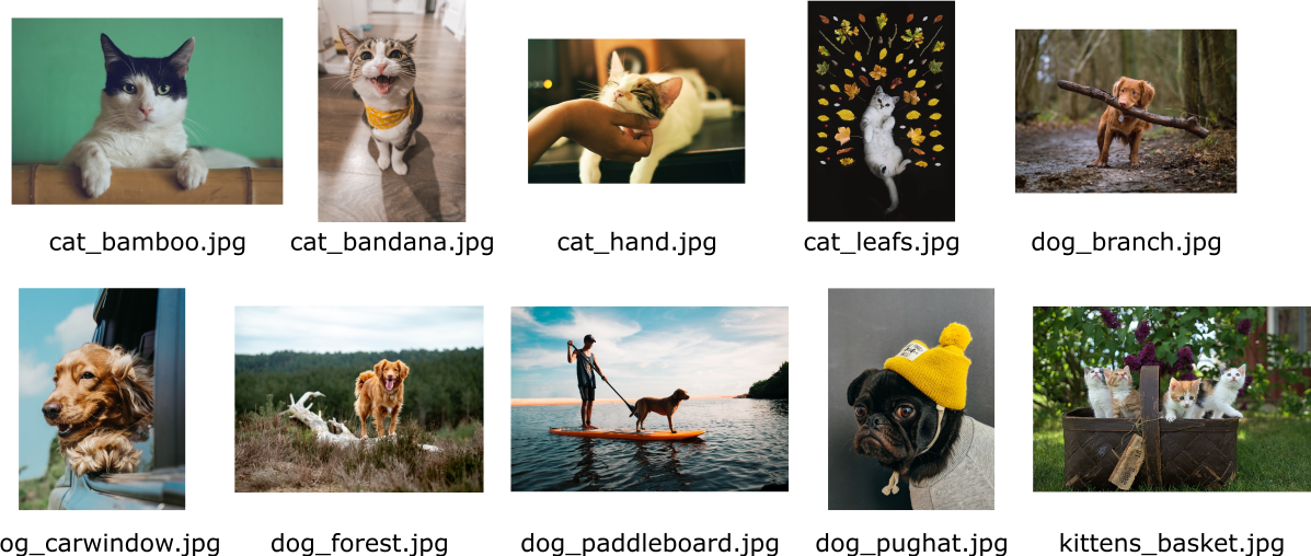
Let’s now take a look at actually making predictions using the model. I chose five cat photos and five dog photos from https://unsplash.com/, and fed them to the model, giving an indication of whether the object is a dog (1) or a cat (0). Some of the photos are not as straight forward, since objects surrounding the animal are present, such as hands, leafs, larger background areas etc and may be relatively hard to classify.
The photos are in the upload_cats_and_dogs folder and were re-named by me to indicate their contents. Since we are not using the image generator, we have to manually reduce the size to our model’s image processing size (150x150 pixels).
import numpy as np
from keras.preprocessing import image

#uploaded = files.upload()
uploaded_filenames = os.listdir(f'{os.getcwd()}\\Data\\upload_cats_and_dogs\\')

for fn in uploaded_filenames:

  # predicting images
  path = os.getcwd() + '\\Data\\upload_cats_and_dogs\\' + fn
  img = image.load_img(path, target_size=(150, 150))

  x = image.img_to_array(img)
  x = np.expand_dims(x, axis=0)
  images = np.vstack([x])

  classes = model.predict(images, batch_size=10)

  print(classes[0])

  if classes[0]>0:
    print(fn + " is a dog")

  else:
    print(fn + " is a cat")
Result:
[0.]
cat_bamboo.jpg is a cat (correct)
[1.]
cat_bandana.jpg is a dog (false)
[0.]
cat_hand.jpg is a cat (correct)
[1.]
cat_leafs.jpg is a dog (false)
[1.]
dog_branch.jpg is a dog (correct)
[2.29507e-14]
dog_carwindow.jpg is a dog (correct)
[1.]
dog_forest.jpg is a dog (correct)
[1.]
dog_paddleboard.jpg is a dog (correct)
[1.]
dog_pughat.jpg is a dog (correct)
[1.]
kittens_basket.jpg is a dog (false)
The pictures I uploaded were not predicted entirely correctly. All the dogs were correctly classified as “dog”, but only two out of five cats were classified “cat”.
Step 7: Evaluate the Training and Validation accuracy
Let’s plot the Training/Validation accuracy and loss as collected during training:
#-----------------------------------------------------------
# Retrieve a list of list results on training and test data
# sets for each training epoch
#-----------------------------------------------------------
acc      = history.history[     'accuracy' ]
val_acc  = history.history[ 'val_accuracy' ]
loss     = history.history[    'loss' ]
val_loss = history.history['val_loss' ]

epochs   = range(len(acc)) # Get number of epochs

#------------------------------------------------
# Plot training and validation accuracy per epoch
#------------------------------------------------
plt.plot  ( epochs,     acc )
plt.plot  ( epochs, val_acc )
plt.title ('Training and validation accuracy')
plt.figure()

#------------------------------------------------
# Plot training and validation loss per epoch
#------------------------------------------------
plt.plot  ( epochs,     loss )
plt.plot  ( epochs, val_loss )
plt.title ('Training and validation loss'   )
Result:
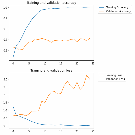
As the graph above shows, we are strongly overfitting our Training Set. Our Training accuracy (in blue) gets close to 100%, while our Validation accuracy (in orange) stalls as ~71%. The validation loss reaches its minimum after only five epochs and then increases steadily.
Since we have a relatively small number of training examples (2000), overfitting should be our greatest concern. Overfitting happens when a model exposed to too few examples learns patterns that do not generalize to new data, i.e., when the model starts using irrelevant features for making predictions.
Overfitting is the central problem in machine learning: given that we are fitting the parameters of our model to a given dataset, how can we make sure that the representations learned by the model will be applicable to data never seen before? How do we avoid learning things that are specific to the training data?
In the next post, I will look at ways to prevent overfitting in this classification model.
Acknowledgements:
Thanks to Lawrence Moroney (Google) by whom this project was inspired (link to notebook on Google CoLab) and Kaggle for their Cats Vs Dogs dataset.