Cats vs. Dogs in TensorFlow Part II
Cats Vs. Dogs computer vision with the TensorFlow API
- Introduction
- Step 1: Transfer Learning
- Step 2: Define Trainable Layers
- Step 3: Download Dataset
- Step 4: Pre-Processing - Image Data Generator and Image Augmentation
- Step 5: Train Model
- Step 6: Evaluate the Training and Validation Accuracy
- Acknowledgements:
Introduction
Given the somewhat mediocre performance of the previous model for Cats Vs Dogs, it seems warranted to implement new tools that promise performance gains. The classification model used previously suffered from overfitting. That means, the training set was learned very well, but probably so well, that the unknown data in the validation set could not be predicted precisely. If a model can only predict well what it has seen before means that it does not “generalize” well.
To improve generalization on the Dogs Vs. Cats set, we can implement two extra measures. Transfer learning, image augmentation, and neuron dropout in some layers. Otherwise, we will keep the setup as before. If details are unclear, read up in Part I
We will follow these steps:
- Transfer Learning
- Define Trainable Layers
- Download Dataset
- Pre-Processing - Image Data Generator and Image Augmentation
- Train Model
- Evaluate the Training and Validation accuracy
If you want to follow along on the Jupyter notebook hosted on GitHub click on this link, otherwise keep on reading.
Step 1: Transfer Learning
Transfer learning is a technique by which we can make use of learned weights of much larger networks. Such networks were trained on millions of images and many classes and are often available to download. What we will do is, download the learned weights of the Inception V3 network and add our own dense layers and outputs on top.
Using the Inception V3 transfer learning enables us to “step on the shoulders of giants” and helps us identify shapes, objects etc. in the images we re-train it on afterwards. We are transferring the learned weights into our own network without the heavy training load of millions of images.
Here, we will download the weights as an .h5 file.
import os
import wget

url = 'https://storage.googleapis.com/mledu-datasets/inception_v3_weights_tf_dim_ordering_tf_kernels_notop.h5'
wget.download(url, out=f'{os.getcwd()}\\Data\\inception_v3_weights_tf_dim_ordering_tf_kernels_notop.h5')
Next, we also have to set up the network itself as the authors of Inception V3 designed it. Luckily, keras has this model already built in in its library. We only have to import it and then fill in the weights from the .h5 file. While training on the cats vs. dogs images, we do NOT want to re-train the entire Inception V3 network. Hence, we set layer.trainable = False
from tensorflow.keras import layers
from tensorflow.keras import Model
from tensorflow.keras.applications.inception_v3 import InceptionV3

# all the weights for the trained Inception V3
local_weights_file = f'{os.getcwd()}\\Data\\inception_v3_weights_tf_dim_ordering_tf_kernels_notop.h5'

# the network shape of Inception V3 is integraded in Keras
pre_trained_model = InceptionV3(input_shape = (150, 150, 3),
                                include_top = False,
                                weights = None)

# combine layout and weights
pre_trained_model.load_weights(local_weights_file)

# make pre-trained model read-only
for layer in pre_trained_model.layers:
  layer.trainable = False
Let’s have a look at the layers of the pre-trained model:
# the Inception V3 is very deep
pre_trained_model.summary()
Result:
Model: "inception_v3"
__________________________________________________________________________________________________
Layer (type)                    Output Shape         Param #     Connected to
==================================================================================================
input_1 (InputLayer)            [(None, 150, 150, 3) 0
__________________________________________________________________________________________________
conv2d (Conv2D)                 (None, 74, 74, 32)   864         input_1[0][0]
__________________________________________________________________________________________________
batch_normalization (BatchNorma (None, 74, 74, 32)   96          conv2d[0][0]
__________________________________________________________________________________________________
activation (Activation)         (None, 74, 74, 32)   0           batch_normalization[0][0]
__________________________________________________________________________________________________
conv2d_1 (Conv2D)               (None, 72, 72, 32)   9216        activation[0][0]
__________________________________________________________________________________________________
batch_normalization_1 (BatchNor (None, 72, 72, 32)   96          conv2d_1[0][0]
__________________________________________________________________________________________________
activation_1 (Activation)       (None, 72, 72, 32)   0           batch_normalization_1[0][0]
__________________________________________________________________________________________________
conv2d_2 (Conv2D)               (None, 72, 72, 64)   18432       activation_1[0][0]
__________________________________________________________________________________________________
batch_normalization_2 (BatchNor (None, 72, 72, 64)   192         conv2d_2[0][0]
__________________________________________________________________________________________________
activation_2 (Activation)       (None, 72, 72, 64)   0           batch_normalization_2[0][0]
__________________________________________________________________________________________________
max_pooling2d (MaxPooling2D)    (None, 35, 35, 64)   0           activation_2[0][0]
__________________________________________________________________________________________________
conv2d_3 (Conv2D)               (None, 35, 35, 80)   5120        max_pooling2d[0][0]
__________________________________________________________________________________________________
batch_normalization_3 (BatchNor (None, 35, 35, 80)   240         conv2d_3[0][0]
__________________________________________________________________________________________________
activation_3 (Activation)       (None, 35, 35, 80)   0           batch_normalization_3[0][0]
__________________________________________________________________________________________________
conv2d_4 (Conv2D)               (None, 33, 33, 192)  138240      activation_3[0][0]
__________________________________________________________________________________________________
batch_normalization_4 (BatchNor (None, 33, 33, 192)  576         conv2d_4[0][0]
__________________________________________________________________________________________________
activation_4 (Activation)       (None, 33, 33, 192)  0           batch_normalization_4[0][0]
__________________________________________________________________________________________________
max_pooling2d_1 (MaxPooling2D)  (None, 16, 16, 192)  0           activation_4[0][0]
__________________________________________________________________________________________________
conv2d_8 (Conv2D)               (None, 16, 16, 64)   12288       max_pooling2d_1[0][0]
.
.
.
.
.
.
.
.
==================================================================================================
Total params: 21,802,784
Trainable params: 0
Non-trainable params: 21,802,784
__________________________________________________________________________________________________
In total, there are almost 100 layers of batch normalizations, 2d convolutions, activations etc. etc…. which makes ~ 22 million parameters.
We will not use the original output of the network, but replace it with our own dense layers and output neurons. We will define the the last / output layer of the Inception network.
# set layer "mixed 7" as end of pre-trained network
last_layer = pre_trained_model.get_layer('mixed7')
print('last layer output shape: ', last_layer.output_shape)
last_output = last_layer.output
Result:
last layer output shape: (None, 7, 7, 768)
Step 2: Define Trainable Layers
As mentioned beforek, we will have to define layers that are attached to the end of the Inception network and are trainable. Four layers will get added. First, a flatten layer that takes the 2d output of the Inception and unravels it into a 1d vector. Second, a trainable fully-connected layer. Third a droput layer, and fourth, an output layer with a single neuron as we had in Part I already.
New is the droput. Droput layers are an additional tool for regularization and will delete random neurons. Many adjacent neurons are thought to be trained with similar values and contribute to overfitting. Setting the droput to 0.2 will make sure that 20% of all neurons in this layer will be canceled. The droput percentage is something to tweak.
from tensorflow.keras.optimizers import RMSprop

# Flatten the output layer to 1 dimension
x = layers.Flatten()(last_output)
# Add a fully connected layer with 1,024 hidden units and ReLU activation
x = layers.Dense(1024, activation='relu')(x)
# Add a dropout rate of 0.2
x = layers.Dropout(0.2)(x)
# Add a final sigmoid layer for classification
x = layers.Dense  (1, activation='sigmoid')(x)

model = Model( pre_trained_model.input, x)

model.compile(optimizer = RMSprop(lr=0.0001),
              loss = 'binary_crossentropy',
              metrics = ['accuracy'])
Step 3: Download Dataset
As in Part I, we have to download the Cats Vs. Dogs data set again and unzip it.
url = 'https://storage.googleapis.com/mledu-datasets/cats_and_dogs_filtered.zip'
wget.download(url, out=f'{os.getcwd()}\\Data\\cats_and_dogs_filtered.zip')
import zipfile

local_zip = f'{os.getcwd()}\\Data\\cats_and_dogs_filtered.zip'

zip_ref = zipfile.ZipFile(local_zip, 'r')

zip_ref.extractall(f'{os.getcwd()}\\Data')
zip_ref.close()
Step 4: Pre-Processing - Image Data Generator and Image Augmentation
As before, we define the train, validation, and paths to the two classes so we can feed them to the Image Data Generator and stream the files into the training process. Here, we will use new parameters for the ImageDataGenerator which will augment the images in the folder on-the-fly. On-the-fly means that the generator applies these augmentations during training without saving data to the hard drive. The modifications taking place are mainly distortions of existing images such as rotation, shearing, mirroring, lateral shifts, and zooms. In short, is a very handy way of vastly increasing the number of training examples without having to take more photos.
from tensorflow.keras.preprocessing.image import ImageDataGenerator

# Define our example directories and files
base_dir = f'{os.getcwd()}\\Data\\cats_and_dogs_filtered'

# create directory names
train_dir = os.path.join( base_dir, 'train')
validation_dir = os.path.join( base_dir, 'validation')

train_cats_dir = os.path.join(train_dir, 'cats') # Directory with our training cat pictures
train_dogs_dir = os.path.join(train_dir, 'dogs') # Directory with our training dog pictures
validation_cats_dir = os.path.join(validation_dir, 'cats') # Directory with our validation cat pictures
validation_dogs_dir = os.path.join(validation_dir, 'dogs')# Directory with our validation dog pictures

# get all training file names
train_cat_fnames = os.listdir(train_cats_dir)
train_dog_fnames = os.listdir(train_dogs_dir)

# Add our data-augmentation parameters to ImageDataGenerator
train_datagen = ImageDataGenerator(rescale = 1./255.,
                                   rotation_range = 40,
                                   width_shift_range = 0.2,
                                   height_shift_range = 0.2,
                                   shear_range = 0.2,
                                   zoom_range = 0.2,
                                   horizontal_flip = True)

# Note that the validation data should not be augmented!
test_datagen = ImageDataGenerator( rescale = 1.0/255. )

# Flow training images in batches of 20 using train_datagen generator
train_generator = train_datagen.flow_from_directory(train_dir,
                                                    batch_size = 20,
                                                    class_mode = 'binary',
                                                    target_size = (150, 150))

# Flow validation images in batches of 20 using test_datagen generator
validation_generator =  test_datagen.flow_from_directory( validation_dir,
                                                          batch_size  = 20,
                                                          class_mode  = 'binary',
                                                          target_size = (150, 150))
Result:
Found 2000 images belonging to 2 classes.
Found 1000 images belonging to 2 classes.
Step 5: Train Model
As previously, we pass the image generators for tain and validation to our model and start it!
history = model.fit(
            train_generator,
            validation_data = validation_generator,
            steps_per_epoch = 100,
            epochs = 20,
            validation_steps = 50,
            verbose = 2)
Result:
Epoch 1/20
100/100 - 27s - loss: 0.4954 - accuracy: 0.7655 - val_loss: 0.6056 - val_accuracy: 0.8500
Epoch 2/20
100/100 - 15s - loss: 0.3829 - accuracy: 0.8315 - val_loss: 0.2152 - val_accuracy: 0.9440
Epoch 3/20
100/100 - 15s - loss: 0.3400 - accuracy: 0.8505 - val_loss: 0.2933 - val_accuracy: 0.9360
Epoch 4/20
100/100 - 15s - loss: 0.3316 - accuracy: 0.8625 - val_loss: 0.1953 - val_accuracy: 0.9570
Epoch 5/20
100/100 - 16s - loss: 0.3227 - accuracy: 0.8615 - val_loss: 0.3282 - val_accuracy: 0.9470
Epoch 6/20
100/100 - 16s - loss: 0.3226 - accuracy: 0.8585 - val_loss: 0.3156 - val_accuracy: 0.9530
Epoch 7/20
100/100 - 15s - loss: 0.3046 - accuracy: 0.8700 - val_loss: 0.3480 - val_accuracy: 0.9470
Epoch 8/20
100/100 - 15s - loss: 0.2785 - accuracy: 0.8750 - val_loss: 0.4184 - val_accuracy: 0.9450
Epoch 9/20
100/100 - 15s - loss: 0.2843 - accuracy: 0.8815 - val_loss: 0.3369 - val_accuracy: 0.9500
Epoch 10/20
100/100 - 15s - loss: 0.2957 - accuracy: 0.8800 - val_loss: 0.4547 - val_accuracy: 0.9430
Epoch 11/20
100/100 - 15s - loss: 0.2685 - accuracy: 0.8970 - val_loss: 0.3231 - val_accuracy: 0.9470
Epoch 12/20
100/100 - 15s - loss: 0.2551 - accuracy: 0.8955 - val_loss: 0.4682 - val_accuracy: 0.9480
Epoch 13/20
100/100 - 16s - loss: 0.2701 - accuracy: 0.8935 - val_loss: 0.3559 - val_accuracy: 0.9540
Epoch 14/20
100/100 - 18s - loss: 0.2842 - accuracy: 0.8865 - val_loss: 0.4018 - val_accuracy: 0.9470
Epoch 15/20
100/100 - 17s - loss: 0.2458 - accuracy: 0.9025 - val_loss: 0.4076 - val_accuracy: 0.9550
Epoch 16/20
100/100 - 16s - loss: 0.2533 - accuracy: 0.9025 - val_loss: 0.3737 - val_accuracy: 0.9620
Epoch 17/20
100/100 - 15s - loss: 0.2465 - accuracy: 0.9080 - val_loss: 0.3398 - val_accuracy: 0.9650
Epoch 18/20
100/100 - 15s - loss: 0.2620 - accuracy: 0.8925 - val_loss: 0.3271 - val_accuracy: 0.9640
Epoch 19/20
100/100 - 15s - loss: 0.2321 - accuracy: 0.9060 - val_loss: 0.3551 - val_accuracy: 0.9670
Epoch 20/20
100/100 - 15s - loss: 0.2470 - accuracy: 0.9000 - val_loss: 0.4488 - val_accuracy: 0.9500
Step 6: Evaluate the Training and Validation Accuracy
Finally we can check what the new implemented tools did to improve the model by plotting the training history. Remember, in the old model Training Accuracy rose to almost 100% after 15 epochs, while the Validation Accuracy stagnated near ~70%.
from matplotlib import pyplot as plt

#-----------------------------------------------------------
# Retrieve a list of list results on training and test data
# sets for each training epoch
#-----------------------------------------------------------
acc      = history.history[     'accuracy' ]
val_acc  = history.history[ 'val_accuracy' ]
loss     = history.history[    'loss' ]
val_loss = history.history['val_loss' ]

epochs   = range(len(acc)) # Get number of epochs

#------------------------------------------------
# Plot training and validation accuracy per epoch
#------------------------------------------------
plt.plot  ( epochs,     acc, label='Training Accuracy' )
plt.plot  ( epochs, val_acc, label='Validation Accuracy' )
plt.legend(bbox_to_anchor=(1.05, 1), loc=2, borderaxespad=0.)
plt.title ('Training and validation accuracy')
plt.figure()

#------------------------------------------------
# Plot training and validation loss per epoch
#------------------------------------------------
plt.plot  ( epochs,     loss, label='Training Loss' )
plt.plot  ( epochs, val_loss, label='Validation Loss' )
plt.legend(bbox_to_anchor=(1.05, 1), loc=2, borderaxespad=0.)
plt.title ('Training and validation loss'   )
Result:
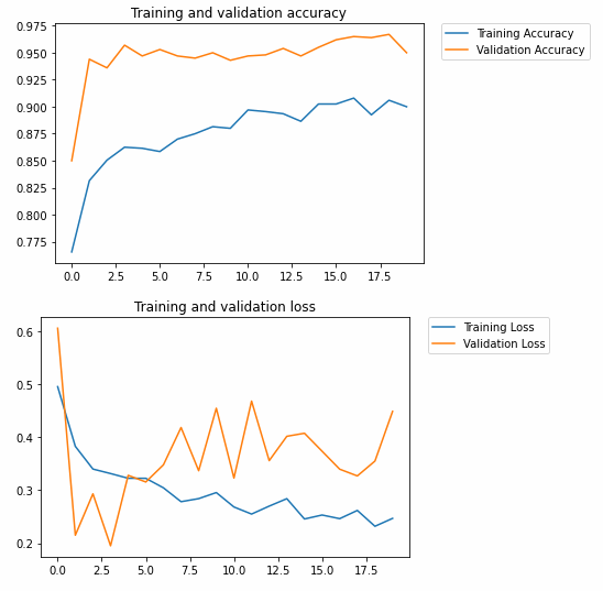
In the new model, the Validation Accuracy (~95%) is even higher than the Training Accuracy (~90%). This is largely a success. Fine-tuning parameters such as the drop out rate and training epochs may be worth a try to modify.
A visible trend in the history losses are increasing too. This means good predictions may be getting worse in higher epochs. Losses keep increasing faster than they are decreases. This remains an issue to be solved.
Acknowledgements:
Thanks to Lawrence Moroney (Google) by whom this project was inspired (link to notebook on Google CoLab) and Kaggle for their Cats Vs Dogs dataset.