Equinor Volve Log ML

Work with real Operator Data!
- Background
- Data
- Problem
- Goal
- Processing
This repository is my exploration on bringing machine learning to the Equinor “Volve” geophysical/geological dataset, which was opened up to the public in 2018.
For more information about this open data set, its publishing licence, and how to obtain the original version please visit Equinor’s Data Village.
The full dataset contains ~ 40,000 files and the public is invited to learn from it. It is on my to-do-list to explore more data from this treasure trove. In fact, the data is not very much explored yet in short the time frame since Volve became open data and likely still holds many secrets. The good thing is that certain data workflows can be re-used from log to log, well to well, etc. So see this as a skeleton blue print with ample space for adaptation as it fits your goals. Some people may even create their bespoke Object-Oriented workflow for processsing automation and best time savings in repetitious work such as this large data set.
The analysis in this post was inspired in parts by the geophysicist Yohanes Nuwara (see here). He also wrote a TDS article see here on the topic, that’s worth your time if you want to dive in deeper!
More on the topic:
- Alfonso R. Reyes Blog: The impact of the Volve dataset
- Agile Scientific Blog: An update on Volve
- Agile Scientific Blog: Big open data… or is it?
The full repository including Jupyter Notebook, data, and results of what you see below can be found here.
Background
The Volve field was operated by Equinor in the Norwegian North Sea between 2008—2016. Located 200 kilometres west of Stavanger (Norway) at the southern end of the Norwegian sector, was decommissioned in September 2016 after 8.5 years in operation. Equinor operated it more than twice as long as originally planned. The development was based on production from the Mærsk Inspirer jack-up rig, with Navion Saga used as a storage ship to hold crude oil before export. Gas was piped to the Sleipner A platform for final processing and export. The Volve field reached a recovery rate of 54% and in March 2016 when it was decided to shut down its production permanently. Reference.
Data
Wireline-log files (.LAS) of five wells:
- Log 1: 15_9-F-11A
- Log 2: 15_9-F-11B
- Log 3: 15_9-F-1A
- Log 4: 15_9-F-1B
- Log 5: 15_9-F-1C
The .LAS files contain the following feature columns:
| Name | Unit | Description | Read More |
|---|---|---|---|
| Depth | [m] | Below Surface | |
| NPHI | [vol/vol] | Neutron Porosity (not not calibrated in basic physical units) | Reference |
| RHOB | [g/cm3] | Bulk Density | Reference |
| GR | [API] | Gamma Ray radioactive decay (aka shalyness log) | Reference |
| RT | [ohm*m] | True Resistivity | Reference |
| PEF | [barns/electron] | PhotoElectric absorption Factor | Reference |
| CALI | [inches] | Caliper, Borehole Diameter | Reference |
| DT | [μs/ft] | Delta Time, Sonic Log, P-wave, interval transit time | Reference |
Problem
Wells 15/9-F-11B (log 2) and 15/9-F-1C (log 5) lack the DT Sonic Log feature.
Goal
Predict Sonic Log (DT) feature in these two wells.
Processing
Imports
import numpy as np
import matplotlib.pyplot as plt
import pandas as pd
import seaborn as sns
import itertools

import lasio

import glob
import os
import md_toc
Load data
LAS is an ASCII file type for borehole logs. It contains:
- the header with detailed information about a borehole and column descriptions and
- the main body with the actual data.
The package LASIO helps parsing and writing such files in python. Reference: https://pypi.org/project/lasio/
# Find paths to the log files (MS windows path style)
paths = sorted(glob.glob(os.path.join(os.getcwd(),"well_logs", "*.LAS")))

# Create a list for loop processing
log_list = [0] * len(paths)

# Parse LAS with LASIO to create pandas df
for i in range(len(paths)):
  df = lasio.read(paths[i])
  log_list[i] = df.df()
  # this transforms the depth from index to regular column
  log_list[i].reset_index(inplace=True)

log_list[0].head()
| DEPTH | ABDCQF01 | ABDCQF02 | ABDCQF03 | ABDCQF04 | BS | CALI | DRHO | DT | DTS | … | PEF | RACEHM | RACELM | RD | RHOB | RM | ROP | RPCEHM | RPCELM | RT | |
|---|---|---|---|---|---|---|---|---|---|---|---|---|---|---|---|---|---|---|---|---|---|
| 0 | 188.5 | NaN | NaN | NaN | NaN | 36.0 | NaN | NaN | NaN | NaN | … | NaN | NaN | NaN | NaN | NaN | NaN | NaN | NaN | NaN | NaN |
| 1 | 188.6 | NaN | NaN | NaN | NaN | 36.0 | NaN | NaN | NaN | NaN | … | NaN | NaN | NaN | NaN | NaN | NaN | NaN | NaN | NaN | NaN |
| 2 | 188.7 | NaN | NaN | NaN | NaN | 36.0 | NaN | NaN | NaN | NaN | … | NaN | NaN | NaN | NaN | NaN | NaN | NaN | NaN | NaN | NaN |
| 3 | 188.8 | NaN | NaN | NaN | NaN | 36.0 | NaN | NaN | NaN | NaN | … | NaN | NaN | NaN | NaN | NaN | NaN | NaN | NaN | NaN | NaN |
| 4 | 188.9 | NaN | NaN | NaN | NaN | 36.0 | NaN | NaN | NaN | NaN | … | NaN | NaN | NaN | NaN | NaN | NaN | NaN | NaN | NaN | NaN |
# Save logs from list of dfs into separate variables
log1, log2, log3, log4, log5 = log_list
# Helper function for repeated plotting
def makeplot(df,suptitle_str="pass a suptitle"):
# Lists of used columns and colors
columns = ['NPHI', 'RHOB', 'GR', 'RT', 'PEF', 'CALI', 'DT']
colors = ['red', 'darkblue', 'black', 'green', 'purple', 'brown', 'turquoise']
# determine how many columns are available in the log (some miss 'DT')
col_counter = 0
for i in df.columns:
if i in columns:
col_counter+=1
# Create the subplots
fig, ax = plt.subplots(nrows=1, ncols=col_counter, figsize=(col_counter*2,10))
fig.suptitle(suptitle_str, size=20, y=1.05)
# Looping each log to display in the subplots
for i in range(col_counter):
if i == 3:
# semilog plot for resistivity ('RT')
ax[i].semilogx(df[columns[i]], df['DEPTH'], color=colors[i])
else:
# all other -> normal plot
ax[i].plot(df[columns[i]], df['DEPTH'], color=colors[i])
ax[i].set_title(columns[i])
ax[i].grid(True)
ax[i].invert_yaxis()
plt.tight_layout() #avoids label overlap
plt.show()
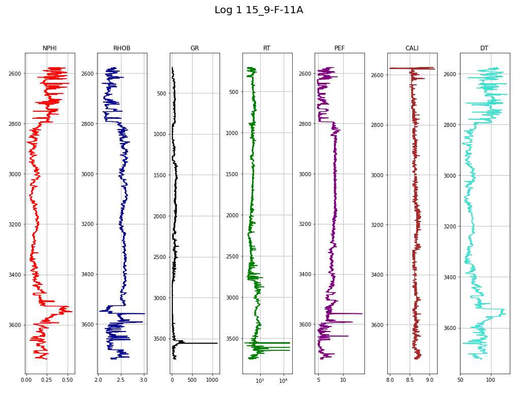
makeplot(log1,"Log 1 15_9-F-11A")
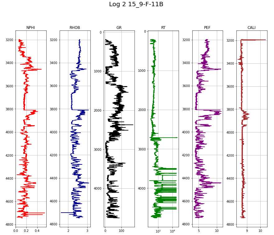
makeplot(log2, "Log 2 15_9-F-11B")
Data Preparation
- The train test split is easy, the data is already partitioned by wells:
- Train on logs 1, 3, and 4.
- Test (validation) on logs 2 and 5.
- There are many NAN values in the logs. The plots above only display the samples that are non-NaN and thus can be used to gauge where they need to be clipped. The NaN are primarily present on top and bottom of each log before readings start. The logs get clipped around the following depths:
- log1 2,600 - 3,720 m
- log2 3,200 - 4,740 m
- log3 2,620 - 3,640 m
- log4 3,100 - 3,400 m
- log5 3,100 - 4,050 m
- Furthermore, the logs contain many more featurs than we need. The correct will get selected for further use, the rest gets discarded.
# Lists of depths for clipping
lower = [2600, 3200, 2620, 3100, 3100]
upper = [3720, 4740, 3640, 3400, 4050]

# Lists of selected columns
train_cols = ['DEPTH', 'NPHI', 'RHOB', 'GR', 'RT', 'PEF', 'CALI', 'DT']
test_cols = ['DEPTH', 'NPHI', 'RHOB', 'GR', 'RT', 'PEF', 'CALI']

log_list_clipped = [0] * len(paths)

for i in range(len(log_list)):

  # Clip depths
  temp_df = log_list[i].loc[
      (log_list[i]['DEPTH'] >= lower[i]) &
      (log_list[i]['DEPTH'] <= upper[i])
  ]

  # Select train-log columns
  if i in [0,2,3]:
    log_list_clipped[i] = temp_df[train_cols]

  # Select test-log columns
  else:
    log_list_clipped[i] = temp_df[test_cols]

# Save logs from list into separate variables
log1, log2, log3, log4, log5 = log_list_clipped
# check for NaN
log1
| DEPTH | NPHI | RHOB | GR | RT | PEF | CALI | DT | |
|---|---|---|---|---|---|---|---|---|
| 24115 | 2600.0 | 0.371 | 2.356 | 82.748 | 1.323 | 7.126 | 8.648 | 104.605 |
| 24116 | 2600.1 | 0.341 | 2.338 | 79.399 | 1.196 | 6.654 | 8.578 | 103.827 |
| 24117 | 2600.2 | 0.308 | 2.315 | 74.248 | 1.171 | 6.105 | 8.578 | 102.740 |
| 24118 | 2600.3 | 0.283 | 2.291 | 68.542 | 1.142 | 5.613 | 8.547 | 100.943 |
| 24119 | 2600.4 | 0.272 | 2.269 | 60.314 | 1.107 | 5.281 | 8.523 | 98.473 |
| … | … | … | … | … | … | … | … | … |
| 35311 | 3719.6 | 0.236 | 2.617 | 70.191 | 1.627 | 7.438 | 8.703 | 84.800 |
| 35312 | 3719.7 | 0.238 | 2.595 | 75.393 | 1.513 | 7.258 | 8.750 | 85.013 |
| 35313 | 3719.8 | 0.236 | 2.571 | 82.648 | 1.420 | 7.076 | 8.766 | 85.054 |
| 35314 | 3719.9 | 0.217 | 2.544 | 89.157 | 1.349 | 6.956 | 8.781 | 84.928 |
| 35315 | 3720.0 | 0.226 | 2.520 | 90.898 | 1.301 | 6.920 | 8.781 | 84.784 |
Next Steps:
Concatenate the training logs into a training df and the test logs into a test df
Assign log/well names to each sample.
Move column location to the right.
# Concatenate dataframes
train = pd.concat([log1, log3, log4])
pred = pd.concat([log2, log5])

# Assign names
names = ['15_9-F-11A', '15_9-F-11B', '15_9-F-1A', '15_9-F-1B', '15_9-F-1C']

names_train = []
names_pred = []

for i in range(len(log_list_clipped)):
  if i in [0,2,3]:
    # Train data, assign names
    names_train.append(np.full(len(log_list_clipped[i]), names[i]))
  else:
    # Test data, assign names
    names_pred.append(np.full(len(log_list_clipped[i]), names[i]))

# Concatenate inside list
names_train = list(itertools.chain.from_iterable(names_train))
names_pred = list(itertools.chain.from_iterable(names_pred))

# Add well name to df
train['WELL'] = names_train
pred['WELL'] = names_pred

# Pop and add depth to end of df
depth_train, depth_pred = train.pop('DEPTH'), pred.pop('DEPTH')
train['DEPTH'], pred['DEPTH'] = depth_train, depth_pred

# Train dataframe with logs 1,3,4 vertically stacked
train
| NPHI | RHOB | GR | RT | PEF | CALI | DT | WELL | DEPTH | |
|---|---|---|---|---|---|---|---|---|---|
| 24115 | 0.3710 | 2.3560 | 82.7480 | 1.3230 | 7.1260 | 8.6480 | 104.6050 | 15_9-F-11A | 2600.0 |
| 24116 | 0.3410 | 2.3380 | 79.3990 | 1.1960 | 6.6540 | 8.5780 | 103.8270 | 15_9-F-11A | 2600.1 |
| 24117 | 0.3080 | 2.3150 | 74.2480 | 1.1710 | 6.1050 | 8.5780 | 102.7400 | 15_9-F-11A | 2600.2 |
| 24118 | 0.2830 | 2.2910 | 68.5420 | 1.1420 | 5.6130 | 8.5470 | 100.9430 | 15_9-F-11A | 2600.3 |
| 24119 | 0.2720 | 2.2690 | 60.3140 | 1.1070 | 5.2810 | 8.5230 | 98.4730 | 15_9-F-11A | 2600.4 |
| … | … | … | … | … | … | … | … | … | … |
| 32537 | 0.1861 | 2.4571 | 60.4392 | 1.2337 | 5.9894 | 8.7227 | 75.3947 | 15_9-F-1B | 3399.6 |
| 32538 | 0.1840 | 2.4596 | 61.8452 | 1.2452 | 6.0960 | 8.6976 | 75.3404 | 15_9-F-1B | 3399.7 |
| 32539 | 0.1798 | 2.4637 | 61.1386 | 1.2960 | 6.1628 | 8.6976 | 75.3298 | 15_9-F-1B | 3399.8 |
| 32540 | 0.1780 | 2.4714 | 59.3751 | 1.4060 | 6.1520 | 8.6976 | 75.3541 | 15_9-F-1B | 3399.9 |
| 32541 | 0.1760 | 2.4809 | 58.3742 | 1.4529 | 6.1061 | 8.6978 | 75.4476 | 15_9-F-1B | 3400.0 |
# Pred dataframe with logs 2, 5 verically stacked
pred
| NPHI | RHOB | GR | RT | PEF | CALI | WELL | DEPTH | |
|---|---|---|---|---|---|---|---|---|
| 30115 | 0.0750 | 2.6050 | 9.3480 | 8.3310 | 7.4510 | 8.5470 | 15_9-F-11B | 3200.0 |
| 30116 | 0.0770 | 2.6020 | 9.3620 | 8.2890 | 7.4640 | 8.5470 | 15_9-F-11B | 3200.1 |
| 30117 | 0.0780 | 2.5990 | 9.5450 | 8.2470 | 7.4050 | 8.5470 | 15_9-F-11B | 3200.2 |
| 30118 | 0.0790 | 2.5940 | 11.1530 | 8.2060 | 7.2920 | 8.5470 | 15_9-F-11B | 3200.3 |
| 30119 | 0.0780 | 2.5890 | 12.5920 | 8.1650 | 7.1670 | 8.5470 | 15_9-F-11B | 3200.4 |
| … | … | … | … | … | … | … | … | … |
| 39037 | 0.3107 | 2.4184 | 106.7613 | 2.6950 | 6.2332 | 8.5569 | 15_9-F-1C | 4049.6 |
| 39038 | 0.2997 | 2.4186 | 109.0336 | 2.6197 | 6.2539 | 8.5569 | 15_9-F-1C | 4049.7 |
| 39039 | 0.2930 | 2.4232 | 106.0935 | 2.5948 | 6.2883 | 8.5570 | 15_9-F-1C | 4049.8 |
| 39040 | 0.2892 | 2.4285 | 105.4931 | 2.6344 | 6.3400 | 8.6056 | 15_9-F-1C | 4049.9 |
| 39041 | 0.2956 | 2.4309 | 109.8965 | 2.6459 | 6.3998 | 8.5569 | 15_9-F-1C | 4050.0 |
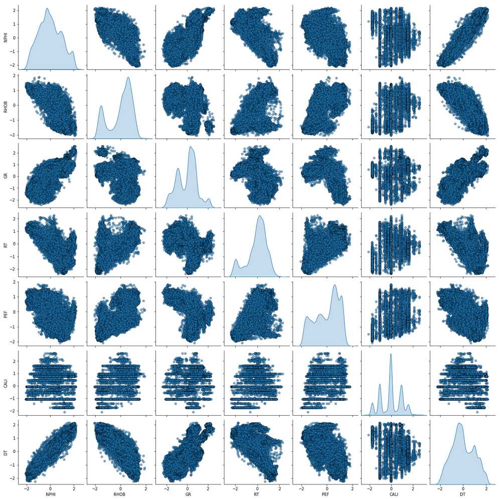
Exploratory Data Analysis
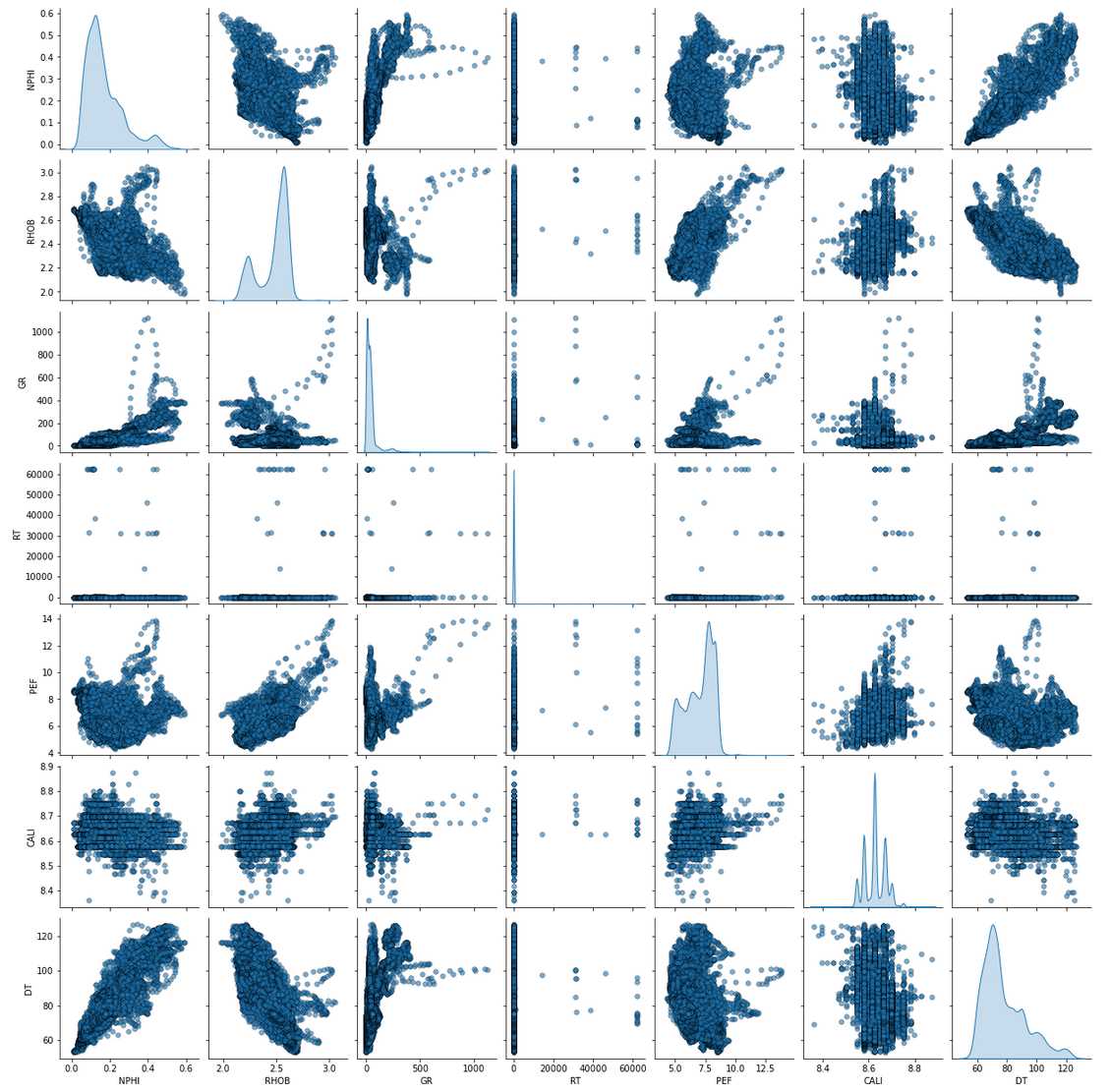
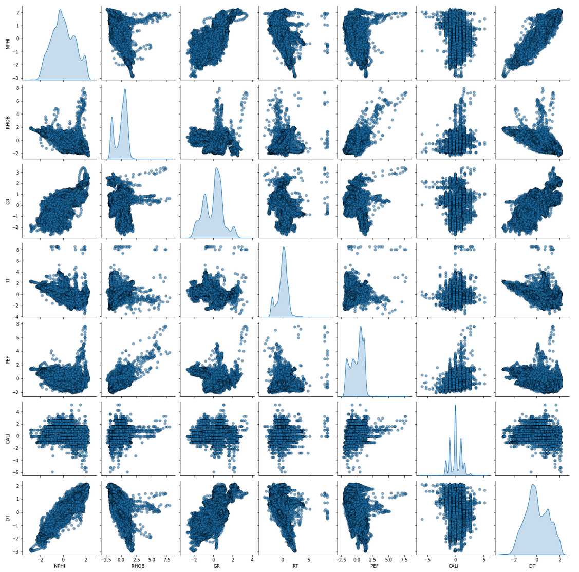
Pair-plot of the Train Data
train_features = ['NPHI', 'RHOB', 'GR', 'RT', 'PEF', 'CALI', 'DT']

sns.pairplot(train, vars=train_features, diag_kind='kde',
             plot_kws = {'alpha': 0.6, 's': 30, 'edgecolor': 'k'})
Spearman’s Correlation Heatmap
train_only_features = train[train_features]

# Generate a mask for the upper triangle
mask = np.zeros_like(train_only_features.corr(method = 'spearman') , dtype=np.bool)
mask[np.triu_indices_from(mask)] = True

# Custom colormap
cmap = sns.cubehelix_palette(n_colors=12, start=-2.25, rot=-1.3, as_cmap=True)

# Draw the heatmap with the mask and correct aspect ratio
plt.figure(figsize=(12,10))
sns.heatmap(train_only_features.corr(method = 'spearman'), annot=True,  mask=mask, cmap=cmap, vmax=.3, square=True)

plt.show()

Transformation of the Train Data
Normalize/transform the dataset:
- Log transform the RT log
- Use power transform with Yeo-Johnson method (except ‘WELL’ and ‘DEPTH’)
# Log transform the RT to logarithmic
train['RT'] = np.log10(train['RT'])

from sklearn.compose import ColumnTransformer
from sklearn.preprocessing import PowerTransformer

# Transformation / Normalizer object Yeo-Johnson method
scaler = PowerTransformer(method='yeo-johnson')

# ColumnTransformer (feature_target defines to which it is applied, leave Well and Depth untouched)
ct = ColumnTransformer([('transform', scaler, feature_target)], remainder='passthrough')

# Fit and transform
train_trans = ct.fit_transform(train)

# Convert to dataframe
train_trans = pd.DataFrame(train_trans, columns=colnames)
train_trans
| NPHI | RHOB | GR | RT | PEF | CALI | DT | WELL | DEPTH | |
|---|---|---|---|---|---|---|---|---|---|
| 0 | 1.702168 | -0.920748 | 1.130650 | -0.631876 | 0.031083 | 0.450019 | 1.588380 | 15_9-F-11A | 2600.0 |
| 1 | 1.573404 | -1.020621 | 1.092435 | -0.736154 | -0.373325 | -1.070848 | 1.562349 | 15_9-F-11A | 2600.1 |
| 2 | 1.407108 | -1.142493 | 1.030314 | -0.758080 | -0.819890 | -1.070848 | 1.525055 | 15_9-F-11A | 2600.2 |
| 3 | 1.260691 | -1.263078 | 0.956135 | -0.784153 | -1.197992 | -1.753641 | 1.460934 | 15_9-F-11A | 2600.3 |
| 4 | 1.189869 | -1.367969 | 0.837247 | -0.816586 | -1.441155 | -2.286221 | 1.367432 | 15_9-F-11A | 2600.4 |
| … | … | … | … | … | … | … | … | … | … |
| 24398 | 0.462363 | -0.279351 | 0.839177 | -0.704005 | -0.910619 | 2.041708 | 0.047941 | 15_9-F-1B | 3399.6 |
| 24399 | 0.439808 | -0.261621 | 0.860577 | -0.694407 | -0.826995 | 1.510434 | 0.043466 | 15_9-F-1B | 3399.7 |
| 24400 | 0.393869 | -0.232335 | 0.849885 | -0.653120 | -0.774093 | 1.510434 | 0.042591 | 15_9-F-1B | 3399.8 |
| 24401 | 0.373838 | -0.176628 | 0.822640 | -0.569367 | -0.782672 | 1.510434 | 0.044596 | 15_9-F-1B | 3399.9 |
| 24402 | 0.351335 | -0.106609 | 0.806807 | -0.535769 | -0.819021 | 1.514682 | 0.052292 | 15_9-F-1B | 3400.0 |
Pair-Plot (after transformation)
sns.pairplot(train_trans, vars=feature_target, diag_kind = 'kde',
             plot_kws = {'alpha': 0.6, 's': 30, 'edgecolor': 'k'})
Removing Outliers
Outliers can be removed easily with an API call. The issue is that there are multiple methods that may work with varying efficiency. Let’s run a few and select which one performs best.
from sklearn.ensemble import IsolationForest
from sklearn.covariance import EllipticEnvelope
from sklearn.neighbors import LocalOutlierFactor
from sklearn.svm import OneClassSVM

# Make a copy of train
train_fonly = train_trans.copy()

# Remove WELL, DEPTH
train_fonly = train_fonly.drop(['WELL', 'DEPTH'], axis=1)
train_fonly_names = train_fonly.columns

# Helper function for repeated plotting

def makeboxplot(my_title='enter title',my_data=None):
    _, ax1 = plt.subplots()
    ax1.set_title(my_title, size=15)
    ax1.boxplot(my_data)
    ax1.set_xticklabels(train_fonly_names)
    plt.show()

makeboxplot('Unprocessed',train_trans[train_fonly_names])
print('n samples unprocessed:', len(train_fonly))
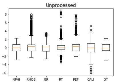
n samples unprocessed: 24,403
Method 1: Standard Deviation
train_stdev = train_fonly[np.abs(train_fonly - train_fonly.mean()) <= (3 * train_fonly.std())]

# Delete NaN
train_stdev = train_stdev.dropna()

makeboxplot('Method 1: Standard Deviation',train_stdev)
print('Remaining samples:', len(train_stdev))
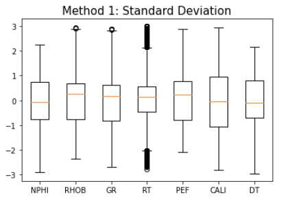
Remaining samples: 24,101
Method 2: Isolation Forest
iso = IsolationForest(contamination=0.5)
yhat = iso.fit_predict(train_fonly)
mask = yhat != -1
train_iso = train_fonly[mask]

makeboxplot('Method 2: Isolation Forest',train_iso)
print('Remaining Samples:', len(train_iso))
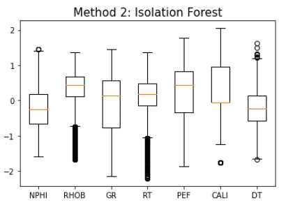
Remaining Samples: 12,202
Method 3: Minimum Covariance Determinant
ee = EllipticEnvelope(contamination=0.1)
yhat = ee.fit_predict(train_fonly)
mask = yhat != -1
train_ee = train_fonly[mask]

makeboxplot('Method 3: Minimum Covariance Determinant',train_ee)
print('Remaining samples:', len(train_ee))
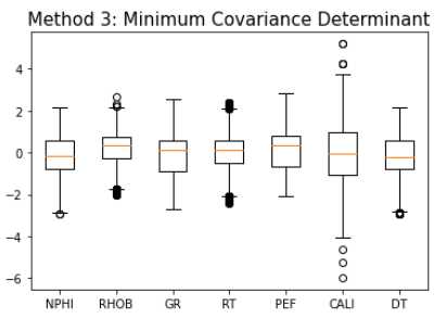
Remaining samples: 21,962
Method 4: Local Outlier Factor
lof = LocalOutlierFactor(contamination=0.3)
yhat = lof.fit_predict(train_fonly)
mask = yhat != -1
train_lof = train_fonly[mask]

makeboxplot('Method 4: Local Outlier Factor',train_lof)
print('Remaining samples:', len(train_lof))
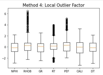
Remaining samples: 17,082
Method 5: Support Vector Machine
svm = OneClassSVM(nu=0.1)
yhat = svm.fit_predict(train_fonly)
mask = yhat != -1
train_svm = train_fonly[mask]

makeboxplot('Method 5: Support Vector Machine',train_svm)
print('Remaining samples:', len(train_svm))
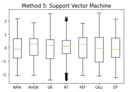
Remaining samples: 21,964
One-class SVM performs best
Make pair-plot of data after outliers removed.
sns.pairplot(train_svm, vars=feature_target,
             diag_kind='kde',
             plot_kws = {'alpha': 0.6, 's': 30, 'edgecolor': 'k'})
Train and Validate
Define the train data as the SVM outlier-removed-data.
# Select columns for features (X) and target (y)
X_train = train_svm[feature_names].values
y_train = train_svm[target_name].values

Define the validation data
train_trans_copy = train_trans.copy()

train_well_names = ['15_9-F-11A', '15_9-F-1A', '15_9-F-1B']

X_val = []
y_val = []

for i in range(len(train_well_names)):
  # Split the df by log name
  val = train_trans_copy.loc[train_trans_copy['WELL'] == train_well_names[i]]

  # Drop name column
  val = val.drop(['WELL'], axis=1)

  # Define X_val (feature) and y_val (target)
  X_val_, y_val_ = val[feature_names].values, val[target_name].values

  X_val.append(X_val_)
  y_val.append(y_val_)

# save into separate dfs
X_val1, X_val3, X_val4 = X_val
y_val1, y_val3, y_val4 = y_val
Fit to Test and Score on Val
from sklearn.metrics import mean_squared_error
from sklearn.ensemble import GradientBoostingRegressor

# Gradient Booster object
model = GradientBoostingRegressor()

# Fit the regressor to the training data
model.fit(X_train, y_train)

# Validation: Predict on well 1
y_pred1 = model.predict(X_val1)
print("R2 Log 1: {}".format(round(model.score(X_val1, y_val1),4)))
rmse = np.sqrt(mean_squared_error(y_val1, y_pred1))
print("RMSE Log 1: {}".format(round(rmse,4)))

# Validation: Predict on well 3
y_pred3 = model.predict(X_val3)
print("R2 Log 3: {}".format(round(model.score(X_val3, y_val3),4)))
rmse = np.sqrt(mean_squared_error(y_val3, y_pred3))
print("RMSE Log 3: {}".format(round(rmse,4)))

# Validation: Predict on well 4
y_pred4 = model.predict(X_val4)
print("R2 Log 4: {}".format(round(model.score(X_val4, y_val4),4)))
rmse = np.sqrt(mean_squared_error(y_val4, y_pred4))
print("RMSE Log 4: {}".format(round(rmse,4)))
R2 Log 1: 0.9526
RMSE Log 1: 0.2338
R2 Log 3: 0.9428
RMSE Log 3: 0.2211
R2 Log 4: 0.8958
RMSE Log 4: 0.2459
This R2 is relatively good with relatively little effort!
Inverse Transformation of Prediction
# Make the transformer fit to the target
y = train[target_name].values
scaler.fit(y.reshape(-1,1))

# Inverse transform  y_val, y_pred
y_val1, y_pred1 = scaler.inverse_transform(y_val1.reshape(-1,1)), scaler.inverse_transform(y_pred1.reshape(-1,1))
y_val3, y_pred3 = scaler.inverse_transform(y_val3.reshape(-1,1)), scaler.inverse_transform(y_pred3.reshape(-1,1))
y_val4, y_pred4 = scaler.inverse_transform(y_val4.reshape(-1,1)), scaler.inverse_transform(y_pred4.reshape(-1,1))
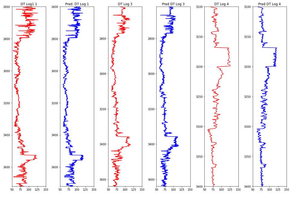
Plot a comparison between train and prediction of the DT feature.
x = [y_val1, y_pred1, y_val3, y_pred3, y_val4, y_pred4]
y = [log1['DEPTH'], log1['DEPTH'], log3['DEPTH'], log3['DEPTH'], log4['DEPTH'], log4['DEPTH']]

color = ['red', 'blue', 'red', 'blue', 'red', 'blue']
title = ['DT Log1 1', 'Pred. DT Log 1', 'DT Log 3', 'Pred DT Log 3',
         'DT Log 4', 'Pred DT Log 4']

fig, ax = plt.subplots(nrows=1, ncols=6, figsize=(15,10))

for i in range(len(x)):
  ax[i].plot(x[i], y[i], color=color[i])
  ax[i].set_xlim(50, 150)
  ax[i].set_ylim(np.max(y[i]), np.min(y[i]))
  ax[i].set_title(title[i])

plt.tight_layout()

plt.show()
Hyperparameter Tuning
This example below is GridSearchCV hyperparameter tuning on Scikit-Learn’s GradientBoostingRegressor, resulting in 31 models playing through all variations.
Different ways of searching hyperparameters are available with automated approaches of narrowing it down in a smarter way.
from sklearn.model_selection import train_test_split

# Define the X and y from the SVM normalized dataset
X = train_svm[feature_names].values
y = train_svm[target_name].values

# Train and test split
X_train, X_test, y_train, y_test = train_test_split(X, y, test_size=0.3, random_state=42)
The grid search will churn for several minutes and the best scoring parameter combination saved printed.
from sklearn.model_selection import GridSearchCV

model = GradientBoostingRegressor()

# Hyperparameter ranges

max_features = ['auto', 'sqrt']
min_samples_leaf = [1, 4]
min_samples_split = [2, 10]
max_depth = [10, 100]
n_estimators = [100, 1000]

param_grid = {'max_features': max_features,
              'min_samples_leaf': min_samples_leaf,
              'min_samples_split': min_samples_split,
              'max_depth': max_depth,
              'n_estimators': n_estimators}

# Train with grid
model_random = GridSearchCV(model, param_grid, cv=3)
model_random.fit(X_train, y_train)

# Print best model
model_random.best_params_
{‘max_depth’: 100,
‘max_features’: ‘sqrt’,
‘min_samples_leaf’: 4,
‘min_samples_split’: 10,
‘n_estimators’: 1000}
Predict Test Wells
Define the Test Data
# Define the test data
names_test = ['15_9-F-11B', '15_9-F-1C']

X_test = []
y_test = []
depths = []

for i in range(len(names_test)):
  # split the df with respect to its name
  test = pred.loc[pred['WELL'] == names_test[i]]

  # Drop well name column
  test = test.drop(['WELL'], axis=1)

  # Define X_test (feature)
  X_test_ = test[feature_names].values

  # Define depth
  depth_ = test['DEPTH'].values

  X_test.append(X_test_)
  depths.append(depth_)

# For each well 2 and 5
X_test2, X_test5 = X_test
depth2, depth5 = depths
Transform Test - Predict - Inverse Transform
# Transform X_test of log 2 and 5
X_test2 = scaler.fit_transform(X_test2)
X_test5 = scaler.fit_transform(X_test5)

# Predict to log 2 and 5 with tuned model
y_pred2 = model_random.predict(X_test2)
y_pred5 = model_random.predict(X_test5)

y = train[target_name].values
scaler.fit(y.reshape(-1,1))

# Inverse transform y_pred
y_pred2 = scaler.inverse_transform(y_pred2.reshape(-1,1))
y_pred5 = scaler.inverse_transform(y_pred5.reshape(-1,1))
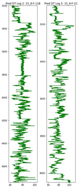
Plot the Predictions
plt.figure(figsize=(5,12))

plt.subplot(1,2,1)
plt.plot(y_pred2, depth2, color='green')
plt.ylim(max(depth2), min(depth2))
plt.title('Pred DT Log 2: 15_9-F-11B', size=12)

plt.subplot(1,2,2)
plt.plot(y_pred5, depth5, color='green')
plt.ylim(max(depth5), min(depth5))
plt.title('Pred DT Log 5: 15_9-F-1C', size=12)

plt.tight_layout()
plt.show()
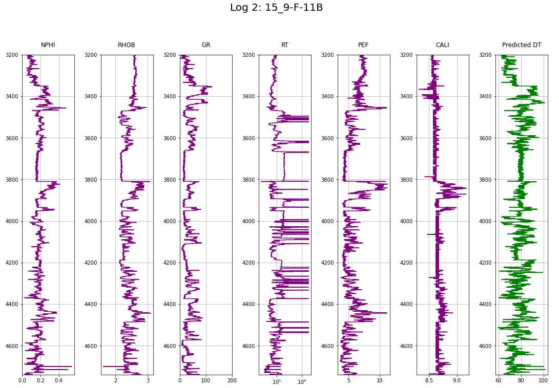
def makeplotpred(df,suptitle_str="pass a suptitle"):
  # Column selection from df
  col_names = ['NPHI', 'RHOB', 'GR', 'RT', 'PEF', 'CALI', 'DT']
  # Plotting titles
  title = ['NPHI', 'RHOB', 'GR', 'RT', 'PEF', 'CALI', 'Predicted DT']
  # plotting colors
  colors = ['purple', 'purple', 'purple', 'purple', 'purple', 'purple', 'green']

  # Create the subplots; ncols equals the number of logs
  fig, ax = plt.subplots(nrows=1, ncols=len(col_names), figsize=(15,10))
  fig.suptitle(suptitle_str, size=20, y=1.05)

  # Looping each log to display in the subplots
  for i in range(len(col_names)):
    if i == 3:
      # for resistivity, semilog plot
      ax[i].semilogx(df[col_names[i]], df['DEPTH'], color=colors[i])
    else:
      # for non-resistivity, normal plot
      ax[i].plot(df[col_names[i]], df['DEPTH'], color=colors[i])

    ax[i].set_ylim(max(df['DEPTH']), min(df['DEPTH']))
    ax[i].set_title(title[i], pad=15)
    ax[i].grid(True)

  ax[2].set_xlim(0, 200)
  plt.tight_layout(1)
  plt.show()
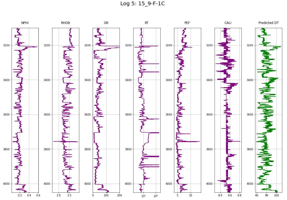
makeplotpred(log2,"Log 2: 15_9-F-11B")
makeplotpred(log5,"Log 5: 15_9-F-1C")