Should you choose to do a PhD?

Is it your cup of tea?
Preamble: I explicitly state that this post is not intended to convince anyone to get a Ph.D. I try to enumerate some common considerations below.
First, should you want to get a Ph.D.? I was in a fortunate position of knowing since when I started my M.Sc. research that I really wanted a Ph.D. Unfortunately it was not for very well gauged and pondered considerations: First, I really liked grad school and learning things, and I wanted to learn as much as possible. Second, I met a many industry Ph.D. who thrived in an industry that is now riding into the sunset. Third, in academia I was surrounded by Ph.D.s and it is taken for granted that you will get a Ph.D. If you are more thorough in making your life’s decisions, What should YOU do?
Many books exist and many a Ph.D. graduate has written about the topic. For example some of the points below were taken from Justin Johnson’s post at Quora: I got a job offer from Google, FB, and MS and laso got accepted into the Ph.D……. Another great Quora threat is: Quora: What is the purpose of doing a Ph.D.. And of course there are many, many subreddits such as r/PhD or many specific career subreddits that often discuss the topic daily.
Assuming that if you are not opting for a Ph.D., another choice for you to consider is joining a medium-to-large company.
Ask yourself if you find the following attributes attractive:
Properties of a Ph.D.
Personal Growth
A Ph.D. is an intense experience of rapid growth -> You soak up knowledge like a sponge. It is a time of personal self-discovery during which you will become a master of managing your own psychology. Many Ph.D. programs offer a high density of exceptionally bright people who have the potential to become your Best Friends Forever.
Expertise
A Ph.D. is probably your only opportunity in life to really delve deeper into a topic and become a recognized leading authority at something within the scientific discourse. You are exploring the edge of humankind’s knowledge, without the burden of lesser distractions or constraints. There is something poetic about that and if you disagree, it could be a sign that Ph.D. is not for you.
Ownership
The research you produce will be yours as an individual and papers with you as first author. Your accomplishments will have your name stamped on them. In contrast, it is much more likely to disappear inside a larger company. A common sentiment is becoming an insignificant member in an anonymous apparatus, a “cog in the machine”.
Exclusivity
Few people make it into top Ph.D. programs. You join a group of a few hundred distinguished individuals contrasted by a few tens of thousands that will join private industry without Ph.D.
Status
While many people in industry tend to belittle Ph.D.s (i.e., “You will work on the matter of a whole Ph.D. every three months in here…”), working towards and eventually getting a Ph.D. degree is societally honored and recognized as an impressive achievement. You also get to be a Doctor; that is great.
Personal Freedom
As a Ph.D. student/candidate you will be your own leader. Bad night and slept in? That works. Skip a day for a vacation? No problem. It is like these companies that have give limitless days off. All that matters is your result and no-one will force you to clock in from 09:00 to 17:00. Some profs (i.e., advisers) might be more or less flexible about it and some companies might be as well.
Maximizing Future Choice
For cutting-edge subjects that just make it out of academia into industry, there is no penalty for obtaining a Ph.D., since you know the latest techniques or even created them. Employers pay big bucks for your talent and brains to invent the next quantum computer etc. For more mature subjects where less revolutionary research happens, lower degrees may be prefered. So if you join a Ph.D. program in a cutting-edge subject, it does not close any doors or eliminate future employment/lifestyle options. You can go from Ph.D. to Anywhere but not the other way Anywhere to Ph.D./Academia/Research. Additionally, it is less likely to get a non-Ph.D. job in academia. Additionally (although this might be quite specific to applied subjects), you are strictly more hirable as a Ph.D. graduate or even as an A.B.D. and many companies might be willing to put you in a more interesting position or with a higher starting salary. More generally, maximal choice for your future is a good path to follow.
Maximizing Variance
You are young and there is really no need to rush. Once you graduate from a Ph.D. you can spend the next tens of years of your life in some company. Choose more variance in your experiences, which will avoid getting pigeon-holed.
Freedom
A Ph.D. will offer you a lot of freedom in the topics you wish to pursue and learn about. You are in charge. Of course, you will have an adviser who will guide you in a certain direction but in general you will have incredible freedom working on your degree than you might find in industry.

Photo by @emilymorter on Unsplash
But wait, there is more…
While the points above sound neutral to positive, it cannot go unsaid that the Ph.D. is a very narrow and specific kind of experience that deserves a large disclaimer:
You will inevitably find yourself working very hard for qualification exams, before conference talks, or submission of the written part near graduation. You need to be accepting of the suffering and have enough mental stamina and determination to deal with the pressure that comes with these crunch times. At some points you may lose track of what day of the week it is and temporarily adopt a questionable diet. You will be tired, exhausted, and alone in the lab on a beautiful, sunny weekend looking at Facebook posts of your friends having fun in nature and on trips, paid with their 5-10 times bigger salaries.
It could happen that you will have to throw away months of your work while somehow keeping your mental health intact. You will live with the fact that months of your time on this Earth were spent on a journal paper that draws limited interest (citations), while your friends participate in exciting startups, get hired at prestigious companies, or get transferred to exotic locations only to become manager over there.
You will experience identity crises during which you will question your life’s decisions and wonder what you are doing with some of the best years of your life. As a result, you can be certain that you can thrive in an unstructured environment in the chase for new discoveries for science. If you are unsure then you should lean towards other pursuits. Ideally you should consider dipping your toe into research projects as an undergraduate or Masters student before before you decide to commit. In fact, one of the primary reasons that research experience is so desirable during the Ph.D. hiring process is not the research itself, but the fact that the student is more likely to know what they are committing to.
Lastly, as a random thought I read and heard that you should only do a Ph.D. if you want remain in to academia. In light of all of the above I would argue that a Ph.D. this is an urban myth and that the Ph.D. has strong intrinsic value of great appeal to many. It is an end by itself, not just a means to some end (e.g., career in academia).

Photo by @homajob on Unsplash
So, you have made the choice. What next?
Getting into a Ph.D. program: (1) references, (2) references, (3) references.
Now how do you get into a good Ph.D. program? The very first step to conquer is quite simple - the by far most important component are strong reference letters.
The ideal scenario is that your professor writes you a glowing letter along the lines of: “X is in top five of students I have ever worked with. X takes initiative, comes up with their own ideas, and can finish a project.”
The worst letter is along the lines of: “X took my class. They are a good student/did well.” That may sound good at first sight, but by academic conventions is not good enough to impress anyone.
A research publication under your belt from a class project (or similar) is a very strong bonus and may often be requested in the application process. But it is not absolutely required, provided you have two/three strong reference letters. In particular note: grades are quite irrelevant, and do not have to be stellar. But you generally do not want them to be out of the usual low. This is not obvious to many students, since many spend a lot of energy on getting good grades, which is a diminishing returns problem. This time spent should be instead directed towards research and thesis work as much and as early as possible. Working under supervision of multiple professors lets them observe your work ethic and skills so that they can confidently write reference letters. As a last point, what will not help you too much is making appearances in the profs offices out of the blue without (recurring?) scheduled meeting times. They are often very busy people and if you do not adhere to appointment schedules, then that may lead to doors closed in your face and even worse, that may backfire on you.
Picking the school
Once you get into some Ph.D. programs, how do you pick the school? Your dream university should:
…be a top university. Not only because it looks good on your résumé and CV but because of less obvious feedback loops. Top universities attract other top students/professors, many of whom you will get to know and work with.
…have a hand full of potential professors you would want to work with. I really do mean a hand full - this is very important and provides a safety net for you if things do not work out with your top choice for any one of dozens of reasons - things in many cases outside of your control, e.g., your dream professor leaves, moves with all the lab equipment but without students, retires, dies (I have seen it a couple of times), has Title IX issues, or spontaneously disappears
…be in a good environment physically. I do not think new students appreciate this enough: you will spend ~5 years of your really good years living in a city that best not be a place you do not really enjoy. Really, this is a long period in your life. Your time in this city consists of much more than just your research and work.
To be continued… Are we done with labeling yet? This is my personal summary from reading Self-supervised learning: The dark matter of intelligence (4th March 2021), which was published on the Facebook AI blog https://ai.facebook.com/blog/. This department at Facebook is dedicated to applied research, but also assembles smart scientists that undertake relatively basic, but ground-braking research. The article is offering an overview of Facebook’s AI-frontier research on self-supervised learning (SSL) in the wake of other papers published by Facebook in the same month DINO and PAWS: Advancing the state of the art in computer vision. Supervised models are specialized on relatively narrow tasks and require massive amounts of carefully labeled data. As we want to expand the capabilities of state-of-the-art models to classify things, “it’s impossible to label everything in the world. There are also some tasks for which there’s simply not enough labeled data […]”. The authors postulate that supervised learning may be at the limits of its capabilities and AI can develop beyond the paradigm of training specialist models. Self-supervised learning can expand the use of specialised training sets to bring AI closer to a generalized, human-level intelligence. Going beyond a specialized training set and forming a common sense from repeated trial-and-error cycles is in essence what humans and animals do. Humans learn without massive amounts of teaching all kinds of possible variants of the same but rather build upon previously learned input. This common sense is what AI research is aspiring to when referring to self-supervised learning and what has remained elusive for a long time. The authors call this form of generalized AI the “Dark Matter” of AI: it is assumed to be everywhere and pervasive in nature, but we can’t see or interact with it (yet?). While SSL is not entirely new. It has found widespread adoption in training models in Natural Language Processing (NLP). Here, Facebook AI uses SSL for Computer Vision tasks and explains why SSL may be a good method for unlocking the “Dark Matter” of AI. Self-supervised learning is trained by signals from the data itself instead of labels. The data in the training set is not a complete set of observations (samples) and thus the missing parts are predicted using SSL. In an ordered dataset such as a sentence or a series of video frames, missing parts or the future/past can be predicted without the use of labels. Since training signals are originating from the dataset itself, the term self-supervised learning is more fitting than the older term “unsupervised learning”. The authors argue that self-supervised learning uses more supervision signals than both supervised and reinforcement learning. In Natural Language Processing, a model is trained by showing it long texts - but no labels. These models are pretrained in a self-supervised phase and then fine-tuned for a use case, such as classifying the topic of a text (see sentiment analysis etc.). When given a sentence with blanked out words, the model can predict the “correct” words. The same concept was tried to apply towards Computer Vision (CV) but so far has never shown the same improvements as in NLP. A large challenge to overcome is the expression of uncertainty for predicted gaps in CV, which was relatively easy in NLP. That is because NLP always works with a finite vocabulary and each word can be given a probability value. Having to design a model for CV requires incorporating accurate representations of errors, which used to be costly in computation and memory. In the past, Facebook’s FAIR workgroup designed a new architecture of Convolutional Networks called RegNet (Regular Network) that solves this issue and efficiently stores billions/trillions of network parameters. It is still impossible to assign error to an infinite number of possible missing frames or patches within a frame, since we do not have a vocabulary as in NLP. However, efficient SSL techniques such as SwAV are improving vision-task accuracy using billions of samples. Photo by @priscilladupreez on Unsplash During NLP’s prediction process the uncertainty is expressed with a softmax function across the entire vocabulary. That means the sum of all vocabulary probabilities add up to 1.0 and the most likely word gets the highest probability assigned. In CV, a frame or patch in a frame out of infinite possibilities is predicted instead of NLP’s discrete vocabulary. We may never be able to assign prediction scores to infinite frames of a high-dimensional continuous space or find techniques to solve this problem. Self-supervised models can be viewed within the framework of energy-based models (EBM). For this model, Siamese networks use two identically architected deep neural networks with shared parameters that encode two images. The networks calculate the two image embeddings, which are compared with each other. The networks are trained to produce low energies, which makes it sometimes difficult to calculate high energies when needed for different images. Several techniques exist to avoid the network to produce very similar embeddings for every sample, which is called “collapse”. Photo by @mrcageman on Unsplash Latent-variable models can be trained with contrastive methods. A good example of contrastive models is the Generative Adverserial Network (GAN) architecture. In SSL, selecting well-chosen pairs of As desribed above, NLP problems are easier to tackle with its finite vocabulary. A latent-variable predictive architecture can be given an observation However, it is very difficult to find maximally incompatible pairs of images (high-dimensional data). So, how could it be possible to increase energy for incompatible candidates? This is a very actively researched field in SSL and are divided into two groups: However, the authors hypothesize that it may be beneficial in the future to combine non-contrastive models with latent variables. Future research will focus on top performing models without requiring large amounts of labeled data. Photo by @vork on Unsplash A new network was trained at Facebook AI called SEER that may bring about a paradigm shift in CV: Supervised learning is at the forefront of everyone’s attention today. Self-supervised methods have been restricted to certain niches such as NLP, where predictions were descrete and finite. Current challenges with bringing Self-supervised methods to CV requires solving problems of calculating probabilities for infinite continuous, hyperdimensional predictions. Siamese networks trained on non-contrasting data is current state-of-the-art to avoid endless training of supervised networks. Facebook released a new, open-source network called SEER that outperforms any other self-supervised network after it was pre-trained on random, un-labeled images. I accidentally dropped a table. Not. Database tables are split up into sub-tables to avoid saving redundant records. This requires the maintenance of more complex systems, but it may be more efficient after all. However, while querying and joining we can combine these tables again. This post contains a number of SQL used for managing values, columns, tables, and databases. Of course, the original tables and outputs are not available here, but the point is providing a lookup for structures and building blocks. New tables can be created directly in SQL syntax. For example: Most common Data Types: PostgreSQL Documentation: DataType table Delete the entire table. List all foreign Keys For Example: For Example: Use DISTINCT to remove duplicate records. Similar as INSERT INTO column, but with additional conditoins. Delete rows selectively where conditions are met. Have you made a type when creating a table? Delete a column in a table. After creation, the datatype of a column can still be modified. Extension of a string lenghth is easy. Shortening the length of a value requires a processing step first. For example, a float type gets rounded first and then cast to integer type. For example, when shortening string entries,a ‘SUBSTRING’ has to be created first selecting the characters from 1 to x. By default, a colum can contain NULL values. A column’s ‘NOT NULL’ flag can be set after the table was created. Remove ‘NOT NULL’. Note: The unique constraint will require a new column be created. Add a primary key serial type. Generate a foreign key column that references a primary key in another table. Assuming a star pattern schema, the central table will get a foreign key added to an central_table_id that refernece the branch_id. For example: Inserting entries into the employees table that violate the foreign key table, e.g. non-existing company, will result in error. Drop / Delete a Foreign Key Column This is two foreign key columns referencing other tables in a many to many relationship. Foreign Keys referencing other tables can be used to prevent entering or deleting data that is not given/referred to in the other table. We can determine what happens to the referenced table if an entry of our foreign key gets deleted. Example: NO ACTION If you delete an entry in table b, the system will raise an error. Example: CASCADE If you delete an entry in table b, all referencing entries in table a will be deleted, too. Use after INSERT, UPDATE, DELETE data manipulation. The tables ‘deleted’ and ‘inserted’ are automatically created by SQL Server. Example 1: AFTER DELETE Example 2: AFTER INSERT, UPDATE The ‘inserted’ is used for both ‘INSERT’ and ‘UPDATE’. Example 3: After INSERT, execute e-mail sending script. Example 4: Differentiate UPDATE and Insert with CASE Write changes into a ClientAuditTable Use instead of INSERT, UPDATE, DELETE data manipulation. Example 1: Instead of updating, raise an error message and send a push email. Example 2: Instead of inserting, check first if condition is met, then resume insert FOR triggers can only be run after, not instead of. That means ‘FOR’ is a synonym for ‘AFTER’. It is impossible to prevent server or database events with ‘INSTEAD OF’, however they can be rolled back with ‘FOR’ The ‘DATABASE’ level includes all tables in the database. Roll back a database-level event with ‘FOR’. Roll back a server-level event with ‘FOR’. Server-level triggers: Database + Table-level triggers (see column ‘parent_class_desc’): Example: Show all disabled triggers The name of a specific trigger has to be known and then can be entered as object_id. Method 1: Method 2: On table level: On database level: On Server level: ‘ALTER TRIGGER’ Altering triggers works with the same syntax as ‘CREATE TRIGGER’, but combines the dropping and creating of a trigger in one step. The ultimate process does not exist. Only compromises. For starting a career as Data Scientist (or moving laterally, pivoting) you need to go through interviews such as for any other role. Either way, Data Science has its very own rules, pitfalls, and pre-conceptions that are hard to navigate. Sometimes, the process is more similar to Software Engineering, sometimes closer to Business. Candidates/applicants want to know what is special about a Data Science interview. Hiring managers want to know which is the right or wrong way to interview. Having had conversations with friends and family in the technology sector, linkedin.com, anonymous platforms such as reddit.com, and teamblind.com, I came to the conclusion that there is no universally right way to interview. This is super important for both hiring managers and candidates to understand. Why? It is all about making compromises. There are no absolutes: Shorter, more succinct interview processes introduce a higher risk of hiring the suboptimal candidate. Longer, more in-depth interview processes, introduce a higher risk of false negatives (i.e., rejecting a candidate who would actually be great for the role), and a higher risk of just rejecting qualified applicants. A strong focus on quizzes / coding tests / quick reaction questions / take-home assignments can introduce a high risk of giving good scores to applicants who either prepared super well how to interview or simply got lucky and knew the answers to those specific questions. Focusing instead only on their work experience introduces a high risk of hiring someone who cannot improvise. Having said that, in my experience there are a couple of universal facts in a statistical sense that really help with interviewing: A history of continuously being productive is with high likelihood an indicator for being productive in the future. Applicants with a history / résumé that lack productivity are unlikely to become productive in a new role. This is, of course, a relatively sweeping judgement, I know. Let me explain. Many candidates look great on paper, had the right classes, know the right things, talk convincingly about their abilities… – but for some reason, when they get hired, would struggle to get things done. Everything would take too long, people overthink things, don’t know when to ask for help, etc. And that is when the red flags showed up (retroactively): The candidates knew all the facts, but had never produced output. Whether in grad school (publications, projects,…) or at work. The ratio of productivity/knowledge is out of balance. According to some people, this is mostly an inherent trait. Some candidates just find ways to get things done, and other candidates find ways to NOT get things done. Many people believe that there is very little you can do as a manager to change that in a person. This leads to the realization that if a candidate who aces every part of the interview but has nothing to show for in his previous roles becomes a concern - unless they have an explanation as to why. Most of the time there is no satisfactory reason why. Hiring managers: Focus on evidence of productivity in candidates. Candidate: Make your résumé scream “I will get stuff done”. Achievements outweigh knowledge. Photo by @magnetme on Unsplash Everyone is going to be compared against a benchmark, but the benchmarks are different. Someone fresh out of a Masters degree is going to get graded on a different scale than someone with two years of experience. But either way, the candidate needs to look productive relative to their peers. Candidates do not need to provide excessive detail to show they were productive. Ideally, a candidate can write/say something along the lines of “Delivered $2M in revenue by implementing a [some ML] model in [language]”. If a professional candidate is not allowed to disclose those details, they can remove the quantities and keep it vaguer. What’s critical is that they provide a cumulative list of projects / impact that looks compelling. If the candidate has worked for an employer for two years, they need to either have one to two really impressive accomplishments, or four to six more moderate/minor ones. They need a combination of volume and impact that stands out. Something candidates often miss: it is not good practice to combine or aggregate multiple projects (e.g., “Delivered $[x]M in value across several projects”). Instead, listing every single project is likely to be more successful. Do not say/write things such as “Collaborated on several cross-department initiatives”. List every single one and what was accomplished in them – even if minor. For example, compare these two lists: vs. Generated $[xxx]K in costs savings by optimizing ad spend across channels using a linear programming approach. Identified $[xxx]K in additional revenue opportunities through targeted price increases. Mitigated COGS increases of [x]% by consolidating volume across multiple brands. Helped leadership identify $[xx]K in redundancies by providing ad-hoc analysis to identify redundancies. What would you prefer as hiring manager? Conversations with DS hiring managers yielded that they are almost surely going to prefer the second list, because it tells them the candidate has generated value in many different ways and times. That means more evidence that proves “I can accomplish things”. As a fresh graduate, it is critical is to make sure to cover all papers, reports, documents, projects, etc. Descriptions to avoid are: And instead break that down into details: Performed literature review (>20 manuscripts) in [something] design, [type of] algorithms and [something] optimization. Conducted weekly research meetings with researchers in the Department of [something]. Prototyped novel model using combination of [language] and [framework]. Delivered monthly status updates to advisor. Focus on detailed accomplishments and results. If possible, provide numbers. Photo by @casparrubin on Unsplash While it is a platitude, it is still a universal truth: “The only constant in workplaces is change.” For many hiring managers very high on the priority list is finding out if someone can learn exactly those things quickly they will need them to do now and in the future. Other hiring managers ask themselves “What would this person do today?”, and then focus on finding people who are doing exactly those things today. If the applicant pool is large (e.g., the manager needs them to code in [language]), then it is a reasonable approach to be very specific. However, if the candidate pool is small (e.g., they need people with experience in one specific algorithm), then things become difficult. This is because the odds of finding someone who is both an excellent interviewee and has that exact experience is miniscule. This is where the search principles come back to the productivity history screening. Hiring managers should put more emphasis on finding productive people than finding people with the exact experience they want. Why? Experience can be acquired. People can learn. Not only that, what they may have to do today may not be what they will be doing half a year in the future. Perhaps that new employee comes in and they themselves are able to suggest a new approach that works better than what was done before, rendering that skill set obsolete. A candidates’ current skill set is largely dictated by their current job, and should not be taken as a fixed, static skill set. When hiring managers consider candidates that have been in a single environment for several years, then they look at the résumé and assume that what the candidate is doing now is just who they are. “Well, this applicant has done a lot of reporting as Data Analyst - not what I we are looking for. We need a Data Scientist building [some type of] models.” And that is the wrong approach. Because what all this indicates is that candidate is doing reports, which is what they need to do in order to do their current job well. So, what can a hiring manager do with a candidate that has done mostly Data Analysis-work but wants a position as Data Scientist training models? Answer: Measure productivity. If the applicant’s previous job was data analytics reporting, then how successful were they at that? Did they differentiate themselves in that field? Did they go above and beyond what others would have done in the role? What experience does the applicant have with modeling - not in this previous role, any time before? How well can they describe that experience? How willing are they to return to it? What experience does the applicant have picking up new skills? In their current role, did they have to learn new technologies or languages? Hiring managers can take the risk-averse position and not even entertain the thought of hiring someone without the exact résumé and experience they are looking for. But they are overwhelmingly likely to miss out on some great candidates. The Unix shell tricks for the Command Line Interface The following writeup contains general bash knowledge I have written down over the years and finally decided to translate into markdown. More flags and examples are found in the internets. Globbing is using wildcards to select multiple files and is similar to regex (see below). Gzipping deletes the original, gunzipping deletes the zipped file Compression levels 1 = weak, 9 = strong Access files while they are still compressed Bzip2: Gzip: Xy: Crating a tarball archive c = create, f = filename View contents of tarball t = view Add/update file to exiting tarball archive (only works uncompressed) u = update Extract tarball archive x = extract Extract single file of tarball archive x = extract with f = filename inside the tarball c = create, z = gzip, j = bzip2, J = xy, f = filename Unzipping .tgz zip r = recursively all subfolders Unlike the other file formats, zipping does NOT automatically delete the uncompressed file. unzip Alternative: Open crontab file with Example 1: Task: Run backup script on first day of each month at 21h. Example 2: Task: Run php script every day at 10 AM. Example 3: Task: Run every hour at minute 0. Crate/overwrite a text file with (string) output contents using Create/append a text file with (string) output contents using Create/overwrite a text containing error message using If no error occurs, nothing will be saved to text file. Create/append a text containing error message using Redirecting to ‘/dev/null’ bit bucket (suppress output) Input data to a command, from file instead of a keyboard. Used with commands that don’t accept file arguments. Translate delete letter l in text ; links commands together and runs sequentially. Inputs and outputs are separate. Redirect output to next input. Show contents of passwd file -> make page scrollable Show all files -> only top 10 -> word count only words -i case sensitive search -r recursive in subfolder files -c counts matches -v invert, show what NOT matches -E extended regex | + ? 1 All lines containing the word cat anywhere on the line. 2 All lines that do not contain (inverse) any of the following characters: sawgtfixk. 3 All lines that start with any 3 letters and the word dig. 4 All lines that end with at least one e. 5 All lines that contain one of the following words: org , kay or tuna. 6 Number count of lines that start with one or no c followed by the string ati. All scripts should begin with a shebang, which defines the path to the interpreter (#!/bin/bash). All scripts should include comments to describe their use (#…). Edit scripts with No spaces before/after = assigning variables. Call variable with $ before variable ($username). $# env. variable with count of arguments passed. $? env. variable with error codes (0=no error). $@ or #* env. variable containing ALL passed arguments. $1 - $9 = explicit call of positional parameters 1-9 Single quotes (‘ ‘). Literal interpretation (variable substitution won’t work). Double quotes (“ “). Variable substitution works. Example: “$var” -> varcontent. Back ticks ( Parenthesis method $(). Content gets fetched from a sub-shell. Example: var=“Today’s date is $(date).” Variables are always considered type=str -> math doesn’t work out of the box. Specify interpreter in first line of script -> comment with shebang! (bash folder) Add access permissions to script file + execute script Single quotes vs double quotes Hello Carol Smith! Hello $username! Script Arguments Input: Hello Carol and Dave! Number of Script Arguments ($#) Input: Hello Carol! Number of arguments: 2. Shell-within-a-shell calculation Converting temperature units (pass °F as parameter) Input: 28 Script creating variables from files Input: The three temperatures were 45, 22, and 32 Scalar comparison operators String Comparison Operators Example 1 If one argument is passed Input: Hello Carol! Number of arguments: 1. Example 2 Input: Apples win! Make your own exit codes and end script there Input: Output: Hello Carol! 0 Indsead of long chains of if/else-statements, case-statements are simpler to write. Feed in filename as script argument ($1) Feed in filename as script argument ($1) cat through the file contents and move or remove the files. Pattern: `for [indexing_var] in [iterable] do [something] done Example 1 Example 2 Loop through parameters and print each parameter Input: Output: Hello Carol! Hello Dave! Hello Henry! Example 3 Loop through parameters and check for alphabetical symbols Input: Output: Hello Carol! Hello Dave! Hello Henry! ERROR: Names must only contain letters. Example 4 A script that will take any number of arguments from the user, and print only those arguments which are numbers greater than 10. Example 5 A script combining for-loop and case-statements to sort files into folders based on contents or remove them. A function with no parameters gets set up with the keyword function and curly braces. Variables defined within a function are always in global scope, unlike other programming languages. Instead, they have to be declared as local. The return option is not for returning data, but for error codes (0 = no error, 1-255 = failure). To get data out of a function, the variable can be echoed and/or declared a global variable. Example 1 Example 2 However, it also works without the keyword. Arguments for functions are handled with The percentage is 745.45% csv kit can do csv processing similarl to Pandas data frames. Install using Python pip Print excel spreadsheet Print excel sheet names with flag -n Excel to csv Excel sheet to csv Print a csv like a markdown table. Similar to the pandas command Print column names with flag -n Print first, third, fifth columns by positional argument Print a column by name Add a group column that traces the original file with flag -g and a group name with flag -n Executes an SQL query on a large variety of SQL databases (e.g., MS SQL, MySQL, Oracle, PostgreSQL, Sqlite) and outputs result to csv. SQLite: starts with Postgres: starts with MySQL: starts with Use SQL syntax compatible with the database Write query in one line with no line breaks Applies SQL statements to one or more csv. Creates an in-memory SQL database that temporarily hosts the Suitable for small to medium files only The sql query must be written in one line without breaks. The order of files in the query and the csv files after that must match. Create tables and insert into tables. Start measuring, find bottlenecks. Writing code a programming language is very flexible. Many solutions will lead you to a goal. But not all the ways of are equally quick in computation and parsimonious in memory allocation. For many applications you won’t really bother with using speedier commands. However, this becomes a consideration when dealing with large datasets (aka Big Data) or you prefer to use serverless services that charge by computation time (e.g., AWS Lambdas). How do we find out what command is more efficient and what is less efficient? You can measure! Timeit: line magic ( Line_Profiler, a module that accepts a function and returns a line-by-line analysis how long each line took to execute and its proportion of overall time. A great way to find bottleneck commands in a function. Memory_Profiler, a memory that accepts a function (imported from a .py file) and delivers a line-by-line analysis of memory usage in MiB. If you want to know more about magic commands and code measurement, check out these articles: An example Jupyter Notebook with all the code of this post can be found here Line Magic Line magic is used for short one-liner measuring. For the first use, execute Default parameters: 44 ns ± 1.45 ns per loop (mean ± std. dev. of 7 runs, 10000000 loops each) Setting flags to set custom parameters for repetitions and number of runs: 40.9 ns ± 0.134 ns per loop (mean ± std. dev. of 10 runs, 1000 loops each) Cell Magic Cell Magic is used to measure multi-line scripts. The same flags can be set for cell magic. 3.33 ms ± 71.1 µs per loop (mean ± std. dev. of 7 runs, 100 loops each) The Line Profiler offers a total run time and additionally detailed measurements how much time each line took to execute, how many times it was executed, and what proportion of the total each line makes up. Use and settings of the Memory Profiler is very similar to the Line Profiler. The “Increment” column shows memory volume gained in each line. The Memory Profiler only works with functions that are imported from .py files in the working directory! If the function is too small to measure, it will show “0.0 MiB”. The decorator is used to automate the timing of a function and we do not have to repeat the timing logic over and over. slow_function took 10 seconds 17.8 ms ± 1.07 ms per loop (mean ± std. dev. of 7 runs, 100 loops each) 194 ns ± 1.06 ns per loop (mean ± std. dev. of 7 runs, 10000000 loops each) Summary: The zip function is multiple magnitudes faster than the loop. The Counter function is part of the ‘collections’ package. 12.4 ms ± 382 µs per loop (mean ± std. dev. of 7 runs, 100 loops each) 4.96 ms ± 26.1 µs per loop (mean ± std. dev. of 7 runs, 100 loops each) Summary: Counter takes only about a third of the loop. 1.98 s ± 23.3 ms per loop (mean ± std. dev. of 7 runs, 1 loop each) 724 ns ± 6.85 ns per loop (mean ± std. dev. of 7 runs, 1000000 loops each) Summary: The difference here is most staggering: almost two seconds for the nested loops and less than one millisecond for the function. 11.7 ms ± 128 µs per loop (mean ± std. dev. of 7 runs, 100 loops each) 8.95 ms ± 280 µs per loop (mean ± std. dev. of 7 runs, 100 loops each) What if you are having trouble with a function executing for longer than expected? You can have a timeout alarm set if it runs longer than a set duration of seconds. The example below makes use of a decorator factory that produced decorators with a variable time for the timeout (seconds). TimeoutError Work with real Operator Data! This repository is my exploration on bringing machine learning to the Equinor “Volve” geophysical/geological dataset, which was opened up to the public in 2018. For more information about this open data set, its publishing licence, and how to obtain the original version please visit Equinor’s Data Village. The full dataset contains ~ 40,000 files and the public is invited to learn from it. It is on my to-do-list to explore more data from this treasure trove. In fact, the data is not very much explored yet in short the time frame since Volve became open data and likely still holds many secrets. The good thing is that certain data workflows can be re-used from log to log, well to well, etc. So see this as a skeleton blue print with ample space for adaptation as it fits your goals. Some people may even create their bespoke Object-Oriented workflow for processsing automation and best time savings in repetitious work such as this large data set. The analysis in this post was inspired in parts by the geophysicist Yohanes Nuwara (see here). He also wrote a TDS article see here on the topic, that’s worth your time if you want to dive in deeper! More on the topic: The full repository including Jupyter Notebook, data, and results of what you see below can be found here. The Volve field was operated by Equinor in the Norwegian North Sea between 2008—2016. Located 200 kilometres west of Stavanger (Norway) at the southern end of the Norwegian sector, was decommissioned in September 2016 after 8.5 years in operation. Equinor operated it more than twice as long as originally planned. The development was based on production from the Mærsk Inspirer jack-up rig, with Navion Saga used as a storage ship to hold crude oil before export. Gas was piped to the Sleipner A platform for final processing and export. The Volve field reached a recovery rate of 54% and in March 2016 when it was decided to shut down its production permanently. Reference. Wireline-log files (.LAS) of five wells: The .LAS files contain the following feature columns: Wells 15/9-F-11B (log 2) and 15/9-F-1C (log 5) lack the DT Sonic Log feature. Predict Sonic Log (DT) feature in these two wells. LAS is an ASCII file type for borehole logs. It contains: The package LASIO helps parsing and writing such files in python. Reference: https://pypi.org/project/lasio/ Next Steps: Concatenate the training logs into a training df and the test logs into a test df Assign log/well names to each sample. Move column location to the right. Normalize/transform the dataset: Outliers can be removed easily with an API call. The issue is that there are multiple methods that may work with varying efficiency. Let’s run a few and select which one performs best. n samples unprocessed: 24,403 Remaining samples: 24,101 Remaining Samples: 12,202 Remaining samples: 21,962 Remaining samples: 17,082 Remaining samples: 21,964 One-class SVM performs best Make pair-plot of data after outliers removed. Define the train data as the SVM outlier-removed-data. R2 Log 1: 0.9526 RMSE Log 1: 0.2338 R2 Log 3: 0.9428 RMSE Log 3: 0.2211 R2 Log 4: 0.8958 RMSE Log 4: 0.2459 This R2 is relatively good with relatively little effort! Plot a comparison between train and prediction of the DT feature. This example below is Different ways of searching hyperparameters are available with automated approaches of narrowing it down in a smarter way. The grid search will churn for several minutes and the best scoring parameter combination saved printed. {‘max_depth’: 100, ‘max_features’: ‘sqrt’, ‘min_samples_leaf’: 4, ‘min_samples_split’: 10, ‘n_estimators’: 1000} Remind me, how did that expression go? The following post consists of notes I had on my drive and I had been returning to over and over to remind me of some concepts and SQL syntax. Of course, the original tables and outputs are not available here, but the point is providing a lookup for structures and building blocks. The CASE statement can create a new column based on multiple conditions in a specified column. The structure always follows The following query creates multiple new columns with a summation aggregate function. For each country calculate the percentage of ties (home=away goals_). Use the Similar as in most languages, SQL can make use of Try/Catch (sometimes called exception/error blocks). It is also possible to have a nested TRY block inside the CATCH block, which lets you attempt a second query if the first failed. Use example: the nested (inner) TRY block could be used to write an error message into a table that the outer TRY failed. The following query writes a message to an ‘error’ table if the outer Try block fails. If that fails, too, then the error details of the inner try are queried. ‘RAISERROR’ lets you define a custom error and parameters. Syntax: While regular subqueries can be calculated on their own, correlated subqueries cannot need results from outer queries. Queries with multiple subqueries will get complicated quickly. Subqueries in Correlated subqueries reference one or more columns in the main query. They dend on information in the main query to run, and thus, cannot be executed on their own. Correlated subqueries are evaluated in SQL once per row of data retrieved - a process that takes a lot more computing power and time than a simple subquery. The following Now it’s getting complicated. Best design such queries from inner to outer. CTEs are declared and executed ahead of the main query and help organizing queries with complicated subqueries. They always precede the main query and go The The empty The following qerry with the Calculate a ranking and also order the query by rank. Note: Assigns the same number to rows with identical values and skips over the next numbers. E.g.: 1,2,3,3,5,6,6,8… The following query calculates the average goals per game and groups by league. The averages are ranked by league. Note: Assigns same number to rows with identical values but does NOT skip over the next numbers. E.g.: 1,2,3,3,4,5,5,6… Generate a column that counts the current The Keywords for sliding windows are The window is supposed to run sum and averages between the current row and the top of the table or bottom of the table. They both arrive at the same cumulative sum, but the way to get there is different. Difference The following query is calculating the Running Total (RT) and Running Aaverage (). The window uses ascending date ordering (smallest date number at top) -> the window goes from top (oldest date) of table to current row. The following query is calculating the RT and RA in descending date ordering (largest date number at top) -> the window goes from current row to bottom (oldest date). Moving average (MA). Calculate a column with the 3-year (2 preceding + current) average. The The following query determins (1) for each year’s Olympics which the gold medal country is and (2) which country is the reigning/last champion country. The These functions do not depend on the current row’s position. The following query fetches the gold-winner athlete and a second column with the first athlete. The order is alphabetically. Fetching the last value is more complicated, since it requires the definition of the Otherwise the last value of the window is the current row, and that’s now what we mean. Window functions can be applied to separate columns into processing sections. This way, it can be avoided that functions leak over from one section into another, e.g. when using The following query partitions the table by gender and avoids the Partition by multiple columns (gender and event). The following query subdivides the ordered medals into three pages. Perform aggregate function analysis on the pages/quantiles. The following query gets the average medals earned in each page. Pivoting with A regular query gets entered into the Original: Pivot by year: ROLLUP() vs CUBE() Use ROLLUP() for hierachical data such as data parts (year, quarter) and don’t wall all possible group-level aggregations. Use CUBE() for all possible group-level aggregations The following query counts medals by country and gender. At the gender group level there is a total row (male+female) using the Group totals by all possible groups with Useful for any function that produces nulls, such as Use in Use in Input Table: Output string: USA, RUS, AUS Merge strings with || CHARLOTTE HUNTER Another example: 1: CHARLOTTE HUNTER Merge strings with posgreSQL’s 1: CHARLOTTE HUNTER Police Academy If just the column string is passed to TRIM(), then all If no trim char string passed, is entered, then Syntax: ’#######[email protected]’, ‘[email protected]\(\)$’ [email protected], moc.goh@egdeh Police Academy, 14, 14 Remember, that SQL indexing starts at 1, not 0! [email protected], 6, 6 LEFT(), RIGHT(): Specify how many characters to be clipped starting from the ends. SUBSTRING()/SUBSTR(): Specify the start index and length. SUBSTRING(): Use functions to determine start/end index with FROM…FOR expression. hedge, hog.com Clip a column to 50 characters but do not clip a word in half. PostgreSQL native casting with two colons Standard SQL casting with A User-Defined Function is the equivalent of a Stored Proceedure. A function can bundle several SQL queries together into a package using 100 Postgre has extensions of the normal Additional features are stemming, fuzzy matching (spelling mistakes), and ranking. Calculate the Levenshtein Distance (number of edits required between two words). 3 Calculate Similarity (0-1) Drop duplicate rows based on specific columns, not the entire rows is duplicated. Use a Common Table Expression (CTE) with a window function ‘PARTITION BY’ that creates a row number per window. Any duplicates will have a row number >2. Then, evaluate the CTE and only keep row numbers = 1. This query selects a timestamp style column and performs arithmetic on it with the Convert integers to time intervals. The Two useful functions are Timestamp parts/fields to extract: Examples for the quarter of the year in a timestamp: 1 1 The following query extracts quarters and years from a timestamp column and sums the payment amount by by quarter and years. The following query extracts the rental duration (rental_days) in a time interval of 90 days starting from 2005-05-01. The 2009-01-01 00:00:00 2009-05-01 00:00:00 The following query truncates to a day and counts the number of entries (rentals) by day. Transactions move around values between owners. For example money between bank accounts. This means a transaction contains a subtraction and addition that both have to succeed. The concept of “Atomic transactions” rolls back a transaction if any of its parts raised an error. SQL has a specific ‘TRAN’ keyword that can be put in a ‘TRY’ block. If the ‘TRAN’ raised an error, the ‘CATCH’ block calls a ‘ROLLBACK TRAN’. With ‘SET XACT_ABORT ON;’ errors in a ‘TRAN’ block will always be rolled back. No ‘TRY’ block needed. Note: ‘THROW’ error still works with XACT_ABORT. It is not necessary to fetch the entire array of a column. We can select specific elements with square brackets. Indexing in PostgresSQL starts with 1, and not 0 as with many other languages. Search for text in ARRAY in specific position. Search for text in any ARRAY position with The SQL query is passed as a single string. The tripple quotation mark wrapping (“””) is useful to have multi-row strings in Python. The table name goes in quotation marks and the SQL server connection has to be passed after the query. Connection URI (Uniform Resource Identifier) for PostgreSQL: postgresql://[user[:password]@][host][:port][/database] Do some column transformations in Spark e.g., convert float to string and split on pattern into multiple columns. Loading into analytical PostgreSQL database Creating a table schema works with [column name] [data-type]. ARRAYS can be created with square brackets. Multiple square brackets are nested arrays. Inserting works with calling the column names if only specific columns are inserted into. Inserting multiple rows into all columns at once can be done without column names, but the order has to match the columns. ARRAYS are inserted with curly braces {} and array elements separated by commas. Which tables are in the system database? Which columns are in the ‘actor’ table and what are their details? Column descriptions are detailed: Available in the distribution ready to be installed. dblink, pg_stat_tatements, pg_trgm Currently installed and ready for use. plpgsql First install and then check if the installation succeeded. Summary from reading the Andreessen Horowitz blog The writeup below are some highlights I wrote for myself. If you find the writeup useful and want to know more, then you should absolutely read the article linked. This is my personal summary from reading The New Business of AI (and How It’s Different From Traditional Software), which was published on the Andreessen Horowitz blog a16z.com, a Silicon Valley venture capital (VC) investor. This VC supported the likes of Skype and Facebook when they were still little known and dozens of others whos digital services we are using in our daily lives. The article is excellently written, and part of the AI in 2020 series. This series is a distillation of dozens of interviews the authors lead with ML tams and thus marks a great resource for machine learning professionals who want deep insights into new AI developments, be it startups or mature companies. And last but not least it helps evaluating the next job opportunities. Most of all, the series is intended by Andreessen Horowitz to support AI companies, a sector in which they are investing heavily. Investors are betting today that AI companies will make a similar return as software companies. However, in many cases that AI companies have a different economic construction than software businesses: Lower gross margins -> heavy cloud infrastructure + human support Scaling problems due to edge cases. Weaker defensive moats -> commoditization of AI models and challenges with data network effects. Consistent pattern in the financial data of AI companies: gross margins 50-60% range, 60-80%+ for SaaS businesses. Early investors pushing AI companies for rapid growth over returns may obscure lower growth rates. AI is going to be a new type of business - after SaaS - and it is clearly different from Software. The differences have to be acknowledged and addressed. Software (including SaaS) can be produced once and sold many times. Benefits are: A) recurring revenue streams, B) high (60-80%+) gross margins, and C) super linear scaling with (rare) network effects, D) ownership of intellectual property (source code) builds defensive moats. Each new project requires dedicated headcount and can be sold exactly once: B) revenue is non-recurring, B) gross margins are lower (30-50%), C) and scaling is linear at best, D) Defensibility is challenging – often based on brand or incumbent account control – because any IP not owned by the customer is unlikely to have broad applicability. Appear to combine elements of both software and services. Most AI applications look + feel like normal software: interfacing with users, managing data, or integrating with other systems. However, at the center is a set of trained data models. Maintaining these models is more like a services business. That is: requiring significant, customer-specific work and input costs beyond typical support and success functions. AI is very demanding on cloud infrastructure: training, inference, and retraining due to data-drift, large file size input data and model transfer across cloud regions are more demanding than traditional software operations. Combined, 25% (or more) of revenue are spent on cloud resources. Manual processing can be cheaper in a company’s early start-up phase. Model complexity is growing at fast rate. 10x data is needed for 2x model precision. CPU/GPUs cannot be accelerated and made cheaper fast enough. Distributed computing solves speed issues, but not costs. Training most of today’s state-of-the-art AI models involves the manual cleaning and labeling of large datasets. This process is laborious, and expensive. For many tasks, especially those requiring greater cognitive reasoning, humans are often plugged into AI systems in real time. The need for human intervention will likely decline as the performance of AI models improves. It’s unlikely that humans will be removed entirely. How much will margins increase with AI fully automated? Reducing human intervention (and their costs) will likely increase cloud costs. New customers increases the work for the ML team when the models have to be adjusted for these new customers -> drawing resources away from new sales. The problem is edge cases. Many AI apps have open-ended interfaces and operate on noisy, unstructured data (e.g., images, NLP). Handling edge cases means endless possible input values. Each new customer deployment is likely to infer on completely new data. AI companies spend time re-training the model for each new customer to eliminate edge cases prior to deployment until accuracy reaches acceptable levels. Startups spend more time + resources for deployment than expected. Identifying challenges in advance can be difficult since traditional prototyping tools (mockups, prototypes, beta tests) do not cover edge cases. Some of the best defensive moats are network effects, high switching costs, and economies of scale. Additionally, branding comes from first to market and near-exclusivity. For AI players, differentiation is harder: New model architectures are developed mostly in open, academic settings. Reference implementations (pre-trained models) are available from open-source libraries, and hyperparameters can be optimized automatically. While data is at the heart of AI, it is often owned by customers, in the public domain, or over time becomes a commodity. Moats for AI companies appear to be shallower than for software and shallower than expected. Reduce model complexity: If possible, share a single model (or set of models) among all customers. It is easier to maintain, faster to roll out, and supports a simpler, more efficient engineering organization. Result: minimize cloud costs. Choose problem domains carefully and narrowly: The minimum viable task for AI models is narrower than expected. Choose problems that are hard for humans but easy for AI. That is high scale, low complexity tasks. Plan for high variable costs: build a business model and Go-To-Market strategy with lower gross margins in mind. Understand the distribution of the model data. Model maintenance and human failover are first-order problems. Measure real variable cost (no hiding in R&D). Make conservative assumptions in financial models (esp. fundraise). Scale and (outside) tech advances may not solve the problem. Embrace services: Building hybrid businesses (software/AI plus service) is harder than pure software, but this approach can provide deep insight into customer needs and yield fast-growing, market-defining companies. Plan for change in the tech stack: AI is still new. Standardized tools are just now being built: tools to automate model training, make inference more efficient, standardize developer workflows. Tightly coupling an application to the current state may lead to an architectural disadvantage in the future. Build defensible: It is unclear whether an AI model or the underlying data is a long-term moat. Good products and proprietary data almost always build good businesses. AI may vitalize old markets. Effective cloud strategies are key. Most AI systems are not like software and such the business works differently. AI businesses scale not as easily, and it is harder to build defensibility. Taken together, that makes AI feel more like a service business. These are unfamiliar patterns, which indicate that AI companies are truly something new, including massive opportunities. Summary from reading the Andreessen Horowitz blog The writeup below are some highlights I wrote for myself. If you find the writeup useful and want to know more, then you should absolutely read the article linked. This is my personal summary from reading Taming the Tail: Adventures in Improving AI Economics, which was published on the Andreessen Horowitz blog a16z.com, a Silicon Valley venture capital (VC) investor. This VC supported the likes of Skype and Facebook when they were still little known and dozens of others whose digital services we are using in our daily lives. The article is excellently written, and part of the AI in 2020 series. This series is a distillation of dozens of interviews the authors lead with ML tams and thus marks a great resource for machine learning professionals who want deep insights into new AI developments, be it startups or mature companies. And last but not least it helps evaluating the next job opportunities. Most of all, the series is intended by Andreessen Horowitz to support AI companies, a sector in which they are investing heavily. AI companies is different from traditional software companies. Often they have lower margins, are harder to scale, and don’t always have strong defensive moats. (…in the presence of long-tailed data distributions) Traditional software is a task of engineering. The specifications of a product are defined and then slowly added to the software - one line of code at a time. AI developers build statistical models, measure them, build a new one, measure, and so on. Until a satisfactory quality threshold was crossed, the AI modeler has to go through this experimentation loop. The article quotes an AI CTO that the process is “closer to molecule discovery in pharma” than engineering. Another issue is that the code written by the AI developer only indirectly influences the output, which adds an additional layer of complexity. It mainly governs how the dataset is processed, but the quality of the outcome is unsure. Many ML natural datasets have a long-tailed (skewed) frequency distribution. The long tail makes up ~70% of the total amount of samples. This makes it when picking randomly much more likely to receive a sample from the tail. Head and Middle, where the most common samples are, receive only 30% of picks. However, the low-frequency samples from the tail are harder to train with supervised learning, while value is relatively low. These long-tail samples are often also called “edge cases” and are much harder to get right. Improving models on the long tail costs a lot of compute resources and thus creates more (cloud) costs than traditional software would cause (3-5x higher). Data has a cost to collect, process, and maintain. That means the larger the long-tailed dataset becomes, the harder it becomes to work with it and more costly, too. The projects actually show “DISeconomies of scale”. While more data to improve a model is often available, the long-taildness also means a diminishing return. AI developers may need 10x more data to achieve a 2x subjective improvement. While computing power becomes cheaper and more available (Moore’s Law), this does not occur with model performance at the moment. Economics of AI are a function of the problem (dataset modeling/characterizing causes computing costs), not part of the technology used (computing efficiency gains). Hence, the approach of the long-tail frequency distribution has to be optimized. First of all, it has to be determined if a long-tailed frequency dataset is there at all. If not, then no ML or DL should be used. Linear or Polynomial Regression will be much more efficient. Logistic Regression and Random Forests are popular because they are A) interpretable, B) scalable, C) computationally efficient. DL may have its use cases in NLP (text generation and understanding), sentiment analysis but accuracy improvement has to be tightly balanced with training and maintenance costs. ML is not always the best solution to everything, which should be very closely evaluated. Heuristic and if/then approaches may be much easier to implement. Serving a single (global) model if there is large customer-segment/region overlap is much cheaper than building multiple models. -> “One size fits all” Tactics to build around the long tail: Componentizing: Train different simpler models to do different jobs concurrently. Example: Couldflare using 7 models to detect 6-7 different bot types attacking websites. Each model is global, and relatively easy to maintain. It is common to observe local problem (data) variation with customers, which do have to be addressed. Effort in modeling is based on the degree of local variation (countries, specific large customers….). Example: streaming services generating playlist models for each country. How to bring the benefits of global models to local problems? Operational best practices to improve AI economics: AI is still in its early years and has not yet crossed the peak of the hype cycle. More efficiency is needed. Structures similar to software development will likely appear Self-Supervised Learning - A recap by Facebook AI

Preface
Introduction
Self-supervised learning is predictive learning
Self-supervised learning for NLP and CV

Modeling the uncertainty in prediction
A unified view of self-supervised methods
x is trained material, which is compared to y. A single energy number tells how compatible x and y are or how likely it is that video clip/photo y follows clip/photo x. Low energy denotes good compatibility, high energy bad compatibility. The smaller the differences in x and y, the lower the energy value will be.Joint embedding, Siamese networks

Contrastive energy-based SSL
x, y that are incompatible to achieve high energies.x, the model must be able to produce a set of multiple compatible predictions. Latent-variable predictive models contain an extra input variable z. This variable z is called latent because its value is never observed. As the latent variable z varies within a set, the output varies over the set of predictions.Non-contrastive energy-based SSL (regularization-based)

Advancing self-supervised learning for vision at Facebook
Summary
SQL Table Management

Making and Deleting Tables
Create Table
CREATE TABLE table_name (
	column1 dtype,
	column2 dtype,
	column3 dtype
);
CREATE TABLE rocktypes (
	ID integer PRIMARY KEY,
	name text NOT NULL,
	type text UNIQUE,
	clevage_angle integer
);
DataType Description text String of any length varchar[ (x) ] Maximum length of n characters char[ (x) ] String of set length n boolean TRUE, FALSE, NULL date, time, timestamp time formats numeric no precision defined integer -2147483648 to 2147483647 Drop Table
DROP TABLE table_name;
Information Schema
List all Tables
SELECT table_name
FROM information_schema.tables
WHERE table_schema = 'public';
List all Columns in a Table
SELECT column_name, data_type
FROM information_schema.columns
WHERE table_name = 'employees' AND table_schema = 'public';
List Table Constraints
SELECT constraint_name, table_name, constraint_type
FROM information_schema.table_constraints
WHERE constraint_type = 'FOREIGN KEY';
Insert Into
Insert a Row
INSERT INTO table_name (existing_column1, existing_column2)
VALUES (val1, val2);
INSERT INTO employee (firstname, lastname, department_shortname)
VALUES (NULL, 'Miller', 'SLS');
Insert a Column
INSERT INTO table_name
SELECT column1
FROM old_table;
INSERT INTO rocktypes
SELECT DISTINCT outcrop, handpiece
FROM samples;

/* double check */
SELECT *
FROM rocktypes;
Update Table
UPDATE connections
SET connections.employee_id = employees.id
FROM employees
WHERE connections.firstname = employees.firstname AND connections.lastname = employees.lastname;
Delete Entries
DELETE FROM organizations
WHERE id = 'ABC';
Alter Table
Rename Column
ALTER TABLE table_name
RENAME COLUMN old_colname TO new_colname;
Add Column
ALTER TABLE table_name
ADD COLUMN id varchar(128);
Drop Column
ALTER TABLE table_name
DROP COLUMN column_name;
Column Type
ALTER TABLE table_name
ALTER COLUMN column_name
TYPE varchar(256);
ALTER TABLE table_name
ALTER COLUMN column_name
TYPE integer
USING ROUND(long_num_value);
ALTER TABLE table_name
ALTER COLUMN column_name
TYPE varchar(16)
USING SUBSTRING(column_name FROM 1 FOR 16)
Set Not Null, Drop Not Null
ALTER TABLE table_name
ALTER COLUMN column_name
SET NOT NULL;
ALTER TABLE table_name
ALTER COLUMN column_name
DROP NOT NULL;
Unique Constraint
ALTER TABLE table_name
ADD CONSTRAINT new_col_name UNIQUE(column_name);
Primary Key Constraint
ALTER TABLE table_name
ADD CONSTRAINT new_col_name PRIMARY KEY(old_col_name);
Primary Key / Add Surrogate Key Column
ALTER Table table_name
ADD COLUMN id serial PRIMARY KEY;
Foreign Key Constraint (1 to n)
ALTER TABLE [central_table]
ADD CONSTRAINT [my_name_for_FKey_constraint] FOREIGN KEY (central_table_id) REFERENCES [branch_table] (branch_id);
ALTER TABLE employees
ADD CONSTRAINT employees_fkey FOREIGN KEY (company_id) REFERENCES companies (id);
ALTER TABLE connections
DROP CONSTRAINT connections_organization_id_fkey;
Foreign Key Constraint (n to m)
CREATE TABLE connections (
    employee_id integer REFERENCES employees (id),
    organization_id varchar(256) REFERENCES organizations (id),
    function varchar(256)
	);
Key Referential Integrity
CREATE TABLE a (
    id integer PRIMARY KEY,
    column_1 varchar(64),
    b_id integer REFERENCES b (id) ON DELETE NO ACTION
	);
CREATE TABLE a (
    id integer PRIMARY KEY,
    column_1 varchar(64),
    b_id integer REFERENCES b (id) ON DELETE CASCADE
    );
ALTER TABLE connections
ADD CONSTRAINT connections_organization_id_fkey FOREIGN KEY (organization_id) REFERENCES organizations (id) ON DELETE CASCADE;
ON DELETE… Description NO ACTION Error CASCADE Delete all referencing entries RESTRICT Error SET NULL Set referencing entry to NULL SET DEFAULT Set referencing entry to default value Triggers
Data Manipulation: AFTER triggers
CREATE TRIGGER TrackDeletedProducts
ON ProductsTable
AFTER DELETE
AS
    INSERT INTO DeletedProducts (Product, Price)
    SELECT Product, Price
    FROM deleted;
CREATE TRIGGER TrackClientHistory
ON ClientTable
AFTER INSERT, UPDATE
AS
    INSERT INTO ClientHistoryTable (Client, ClientID, Address, PhoneNumber)
    SELECT Client, ClientID, Address, PhoneNumber, GETDATE()
    FROM inserted;
CREATE TRIGGER NewClientPushEmail
ON ClientTable
AFTER INSERT
AS
    EXECUTE SendNotification @RecipientEmail = '[email protected]'
                            ,@EmailSubject = 'New Client Signup'
                            ,@EmailBody = 'A new client just signed up with us.';
CREATE TRIGGER ClientAudit
ON Orders
AFTER INSERT, UPDATE, DELETE
AS
    DECLARE @Insert BIT = 0;
    DECLARE @Delete BIT = 0;
    IF EXISTS (SELECT * FROM inserted) SET @Insert = 1;
    IF EXISTS (SELECT * FROM deleted) SET @Delete = 1;
    INSERT INTO ClientAuditTable (TableName, EventType, UserAccount, EventDate)
    SELECT 'Orders' AS TableName
           ,CASE WHEN @Insert = 1 AND @Delete = 0 THEN 'INSERT'
                 WHEN @Insert = 1 AND @Delete = 1 THEN 'UPDATE'
                 WHEN @Insert = 0 AND @Delete = 1 THEN 'DELETE'
                 END AS Event
           ,ORIGINAL_LOGIN() AS UserAccount
           ,GETDATE() AS EventDate;
Data Manipulation: INSTEAD OF triggers
CREATE TRIGGER PreventProductsUpdate
ON Products
INSTEAD OF UPDATE
AS
    DECLARE @EmailBodyText NVARCHAR(50) =
                        (SELECT 'User ' + ORIGINAL_LOGIN() + ' tried to update the Products table.');

    RAISERROR ('Updates on "Products" table are not permitted.', 16, 1);

    EXECUTE SendNotification @RecipientEmail = '[email protected]'
                            ,@EmailSubject = 'User tried to update Products'
                            ,@EmailBody = @EmailBodyText;
CREATE TRIGGER ConfirmInventory
ON OrderTable
INSTEAD OF INSERT
AS
    IF EXISTS (SELECT * FROM inventory AS iv
               INNER JOIN  inserted  AS is ON  is.Product = iv.Product
               WHERE iv.Quantity  < is.Quantity )
    RAISEERROR ('You cant order higher quantities than there is in the inventory.', 16, 1);

    ELSE
        INSERT INTO dbo.OrderTable (Client, Product, Quantity, Date, Total)
        SELECT Client, Product, Date, Total FROM inserted;
Data Definition: FOR triggers
CREATE TRIGGER TrackTableChanges
ON DATABASE
FOR CREATE_TABLE,
    ALTER_TABLE,
    DROP_TABLE
AS
    INSERT INTO TablesLog (EventData, User)
    VALUES (EVENTDATA(), USER);
CREATE TRIGGER PreventTableDrop
ON DATABASE
FOR DROP_TABLE
AS
    RAISERROR ('DROP is not allowed.', 16, 1);
    ROLLBACK;
CREATE TRIGGER PreventDatabaseDrop
ON ALL SERVER
FOR DROP_DATABASE
AS
   PRINT 'You are not permitted to drop databases.';
   ROLLBACK;
Listing all triggers and trigger events in the system
SELECT * FROM sys.server_triggers;

SELECT * FROM sys.server_trigger_events;
SELECT * FROM sys.triggers;

SELECT * FROM sys.trigger_events;
SELECT name,
	   object_id,
	   parent_class_desc
FROM sys.triggers
WHERE is_disabled = 1;
Viewing a specific trigger
SELECT definition
FROM sys.sql_modules
WHERE object_id = OBJECT_ID ('PreventTableDrop');
SELECT OBJECT_DEFINITION (OBJECT_ID ('PreventTableDrop'));
Listing all server, DB, and table triggers with definitions
SELECT name AS TriggerName,
       parent_class_desc AS TriggerType,
       create_date AS CreateDate,
       modify_date AS LastModifiedDate,
       is_disabled AS Disabled,
       is_instead_of_trigger AS InsteadOfTrigger,
       OBJECT_DEFINITION  (object_id)
FROM sys.triggers
UNION ALL
SELECT name AS TriggerName,
       parent_class_desc AS TriggerType,
       create_date AS CreateDate,
       modify_date AS LastModifiedDate,
       is_disabled AS Disabled,
       0 AS InsteadOfTrigger,
       OBJECT_DEFINITION  (object_id)
FROM sys.server_triggers
ORDER BY TriggerName;
Disable / Enable / Drop / Alter Triggers
DISABLE TRIGGER PreventProductsUpdate;

ENABLE TRIGGER PreventProductsUpdate;

DROP TRIGGER PreventProductsUpdate;
DISABLE TRIGGER PreventTableDrop
ON DATABASE;

ENABLE TRIGGER PreventTableDrop
ON DATABASE;

DROP TRIGGER PreventTableDrop
ON DATABASE;
DISABLE TRIGGER PreventDatabaseDrop
ON ALL SERVER;

ENABLE TRIGGER PreventDatabaseDrop
ON ALL SERVER;

DROP TRIGGER PreventDatabaseDrop
ON ALL SERVER;
ALTER TRIGGER PreventDatabaseDrop
ON ALL SERVER
FOR DROP_DATABASE
AS
   PRINT 'You are ABSOLUTELY NOT permitted to drop databases.';
   ROLLBACK;
Data Science Hiring Theory

Interview Style
Productivity and Knowledge
Summary

Graduate and Professional Productivity History
Professional
Graduates
Summary

Current Skill Set vs. Learning
Lateral Transfers
Summary
BASHing the Linux console

Important Commands / Apps
Name Name Description Description Flags Example ls, ll list short, list long Display the contents of the current directory -> dir sizes fake ls [dir] long description -l ls -l [dir] human-readable file-sizes -h ls -h [dir] sort by modification time -t ls -t [dir] all hidden paths/dirs -a ls -a [dir] all files and dirs, no subdir contents -d ls -d [dir] all files and dirs, with sub-directories (recursive) similar to “find” or “tree” -R ls -R [dir] sort by extension -X ls -lX [dir] sort by size -S ls -S [dir] reverse sorting -r ls -r [dir] tree prints graphic representation of files and sub-directories (non-std app) tree [directory] root needs sudo privileges sudo tree -F / tree depth, level of recursion -L sudo tree -L 2 / du disk usage print dir content like “ls -lh [dir]”, but with real dir sizes pwd print working directory shows currently set working directory cd change directory changes to a different directory cd [dir] ../.. root dir ~ logged-in user’s home directory . current directory .. parent directory cat concatenate view contents of single file cat [File] view contents of multi files cat [File1] [File2] viewing a file’s content that doesn’t exit yet creates it. cat > [File] cut removes sections from a text file cp copy copies one or multi files, warning: if dest-file exists then it is overwritten cp [Src-file] [Dest-file] directory copy (recursively) -r cp -r [Src-dir] [Dest-dir] copy files to dir cp [Src-file1] [Src-file2] [Dest-dir] mv move move or rename mv [filename] [dest-dir] inform overwrite -i mv -i [file] [new_file] mkdir make directory create a new directory mkdir [newdir] new dir within new dir: mkdir -p [newdir1]/[newdir2] touch creates empty file or updates modification date touch [file1] [file2] [file3] avoid create file if not exists -c touch -c [file] echo print to terminal echo [string] write to file (overwrites previous content) echo hello > file.txt wc word count count number of words -w wc -w [file] count number of lines -l wc -l [file] passwd password changes a user’s password rm remove delete a file OR directory remove dir with sub-dirs -r rm -r [myfolder] remove with inform y/n prompt -i rm -i [myfile] rmdir remove directory deletes a directory, by default only empty dirs rmdir [directory] more view text files one screen at a time (superseded by ‘less’) less views text files, allows scrolling up and down a line or page at a time whereis display the file path to a specified program and related manual files head show the first n lines of a text file head -n 5 [file] tail show the last few lines of a file tail -n 5 [file] sort order line by line (default alphabetical) sort [file] numerical order -n sort -n [file] reverse order -r sort -r [file] tr translate replace or removes characters tr “[:lower:]” “[:upper:]” chmod changes a file permissions (read, write, execute) grep g/re/p search within a file (global regular expression print) case sensitive search -i recursive in subfolder files -r counts matches -c invert, show what NOT matches -v $ grep -v “[sawgtfixk]” [file] extended regex + ? -E grep -E “e+$” [file] find search for file in in home dir find ~ -name [file] search in current dir find . -name [file] find all files ending with number find ~ -name “*[0-9]” locate search for file in index database (update db with sudo updatedb) man open manual page of a command man [command] info open info page of a command info [command] sed works on lines (modifies words or other parts of lines, inserts, deletes) awk work on records with fields which show path of an executable specified in PATH variable which netcat expr expression integer math (not supported in native bash) expr 4 + 1 echo $((4+1)) bc basic calculator decimal-place math, default rounded to 0 decimal places echo “4.1 + 2.3” | bc define decimal places echo “scale=3; 10/3” | bc Globbing
* any number of any character, including no characters. Example: ls question20*3? any ONE character. Example: ls question?3[] class/range of characters. Example: ls file[1-3]^ excluding. Example: ls file[^a][:digit:] digits. Example: ls file[[:digit:]a][:alpha:] alphabetical[:alnum:] alphabetrical + numerical (digits)[:blank:] space, tabs[:space:] space, tabs[:cntrl:] backspace, bell, NAK, escape[:lower:] lowercase[:upper:] uppercase[:punct:] punctuation, period, comma, semicolon, exclamation mark, ampersand[:print:] all printable symbols = alphabetical + numerical + space[:xdigit:]hexadecimalCompression
bzip2, gzip, xy
bzip2 [file]` --> `bunzip2 [file2.bz2]

gzip [file]` –> `gunzip [file3.gz]

xz [file]` --> `unxz [file.xz]
gzip -1 [file]` or `gzip -9 [file]
bzcat, bzgrep,bzdiff, bzless, bzmorezcat, zgrep, zdiff, zless, zmorexycat, xygrep,xydiff, xyless, xymoretar archives
tar -cf [new-tar-dir.tar] [file/dir-worked-on 1] [file/dir-worked-on 2]
tar -tf [file.tar]
tar -uf [file.tar] [file/dir-worked-on 1] [file/dir-worked-on 2]
tar -xf [file.tar]
tar -xf [file.tar] [compression/hosts.gz]
Compressed tar archives (double ending .tar.gz or .tgz)
tar -czf gzip.tar.gz [file/dir-worked-on 1] [file/dir-worked-on 2]

tar -cjf bzip2.tar.bz2 [file/dir-worked-on 1] [file/dir-worked-on 2]

tar -cJf xz.tar.xz [file/dir-worked-on 1] [file/dir-worked-on 2]
gunzip [archive.tgz]

tar xf [archive.tar]
Managing zip files
zip -9 [zipfile.zip][file-worked-on] # 0-9 compression level

zip -r [zipfile.zip] [file/dir-worked-on 1] [file/dir-worked-on 2]
rm -rf [file/dir-worked-on 1]
unzip [zipfile.zip]Cron jobs
crontab -l List all cron jobscrontab -e Edit list of cron jobs, select editornano crontab or vim crontab.crontab -r Delete the current cron jobsnano /etc/crontab
* * * * * /path/to/command arg1 arg2
* * * * * /root/backup.txt
Increment Range first * minutes [0-59] second * hours [0-23] third * day [0-31] tourth * month [0-12] fifth * day of week [0-7] Examples
0 21 1 * * /path/to/script/backup-script.sh
0 10 * * * /path/to/myphpscript.php
0 * * * * /path/to/myphpscript.php
Redirecting input/output/error IO
Keyboard input (stdout, channel 0)
Screen print (stdout, channel 1)
>echo "Hello World!" > text.txt
>>echo "Hello to you too!" >> text.txt
Error (stderr, channel 2)
2>find /usr games 2> text-error.txt
2>>sort /etc 2>> text-error.txt
sort /etc 2> /dev/null
Substituting keyboard input with file contents
cat < text.txt
tr -d "l" < text.txt
Combo redirects (channel 1 screen & channel 2 error)
find /usr admin &> newfile.txt
Command chains
Sequential runs in a command line with ;
Piping | redirect output to next command as input
cat /etc/passwd | less
ls -l | head | wc -w
Redirect output only if successful
&& links commands together, but only runs the 2nd command if the 1st succeeds.csvlook SpotifyData_All.csv && csvstat SpotifyData_All.csv
Grep - searching within files
grep “[regex-term]” [file]

grep “exact-string” /etc/passwd
Regex for grep and more
Expression Description . any char except newline [abcABC] match any char in brackets [^abcABC] match any char except the ones in brackets [a-z] match any char in range [^a-z] match any char except in range sun|moon or ^ start of line $ end of line * Zero or more of the preceding pattern (requires -E) + One or more of the preceding pattern (requires -E) ? Zero or one of the preceding pattern (requires -E) Examples
grep "cat" /usr/share/hunspell/en_US.dic
grep -v "[sawgtfixk]" /usr/share/hunspell/en_US.dic
grep "^...dig" /usr/share/hunspell/en_US.dic
grep -E "e+$" /usr/share/hunspell/en_US.dic
grep -E "org|kay|tuna" /usr/share/hunspell/en_US.dic
grep -cE "^c?ati" /usr/share/hunspell/en_US.dic
Writing / executing bash scripts
cat -n [script.sh] (n=line numbers)` `). Content gets fetched from a sub-shell.echo 'echo "Hello World!"' > new_script.shecho '#!/bin/bash \n echo "Hello World!"' > new_script.shchmod +x [new_script.sh]Examples
#!/bin/bash

username=”Carol Smith”
echo "Hello $username!"
echo ‘Hello $username!’
new_script.sh Carol Dave#!/bin/bash
username1=$1
username2=$2
echo "Hello $username1 and $username2!"
new_script.sh Carol Dave#!/bin/bash
username=$1
echo "Hello $username!"
echo "Number of arguments: $#."
#!/bin/bash

model1=87.56
model2=89.20
echo “Total score is $(echo $model1 + $model2 | bc)”
echo “Average score is $(echo ‘scale=2; ($model1 + $model2) / 2’ | bc)”
tempconverter.sh 84#!/bin/bash
temp_f=$1
temp_f2=$(echo "scale=2; $temp_f - 32" | bc)
temp_c=$(echo "scale=2; $temp_f2 * 5 / 9" | bc)
echo $temp_c
pull_temp_files.sh#!/bin/bash
temp_a=$(cat temps/region_A)
temp_b=$(cat temps/region_B)
temp_c=$(cat temps/region_C)
echo "The three temperatures were $temp_a, $temp_b, and $temp_c"
If-conditions
Operators
-eq equal (=)-ne not equal (!=)-gt greater than (>)-ge greater or equal (>=)-lt less than (<)-le less or equal(<=)abc == abc trueabc == ABC false1 == 1 true1+1 == 2 falseExamples
[ $# -eq 1 ], then echo greeting, else raise error, finish if, print $#new_script.sh Carol#!/bin/bash
if [ $# -eq 1 ]
then
username=$1
echo "Hello $username!"
else
echo "Please enter only one argument."
fi
echo "Number of arguments: $#."
guided1.sh 3 0#!/bin/bash
fruit1=Apples
fruit2=Oranges
if [ $1 -lt $# ]
then
echo "This is like comparing $fruit1 and $fruit2!"
elif [ $1 -gt $2 ]
then
echo "$fruit1 win!"
else
echo "$fruit2 win!"
fi
Exit codes
script.sh Carol#!/bin/bash
# A simple script to greet a single user.
if [ $# -eq 1 ]
then
username=$1
echo "Hello $username!"
exit 0
else
echo "Please enter only one argument."
exit 1
fi
echo "Number of arguments: $#." #never executed, since exited before
echo $? check exit codeCase-conditions
#!/bin/bash

case $1 in
	# Match on all months with OR pipes
	January|March|May|July|September|November)
	echo "It is an odd month!";;

	# Match on all even months
	February|April|June|August|October|December)
	echo "It is an even month!";;

	# Default case if no match (i.e., else)
	*)
	echo "Not a month!";;
esac
#!/bin/bash

case $(cat $1) in
	*Frankfurt*)
	mv $1 frankfurt/ ;;

	*Berlin*)
	rm $1 ;;

	*Hamburg*)
	mv $1 "SPECIAL_$1" ;;

	# Defaultcase if no match
	*)
	echo "No city found" ;;
esac
For-loops
Examples
#!/bin/bash

FILES="/usr/sbin/accept /usr/sbin/pwck/ usr/sbin/chroot"

for file in $FILES
do
	ls -lh $file
done
friendly2.sh Carol Dave Henry#!/bin/bash
# if there are no parameters passed
if [ $# -eq 0 ]
then
echo "Please enter at least one user to greet."
exit 1
else
for username in $@
do
echo "Hello $username!"
done
exit 0
fi
friendly2.sh Carol Dave Henry#!/bin/bash
if [ $# -eq 0 ]
then
echo "Please enter at least one user to greet."
exit 1
else
for username in $@
do
echo $username | grep "^[A-Za-z]*$" > /dev/null
# if the line above produced an error code
if [ $? -eq 1 ]
then
echo "ERROR: Names must only contain letters."
exit 2
else
echo "Hello $username!"
fi
done
exit 0
fi
friendly2.sh 42 Carol Dave Henryecho $? check number of passed arguments 2#!/bin/bash
for arg in $@
do
# strip all numerical symbols
echo $arg | grep "^[0-9]*$" > /dev/null
# if the above produced NO error code
if [ $? -eq 0 ]
then
if [ arg -lt 10 ]
then
echo $arg
fi
fi
done
#!/bin/bash

# loop through files in folder
for file in model_output/*
do
    # cat into file's content
    case $(cat $file) in

		# Matched tree models are moved
		*"Random Forest"*|*GBM*|*XGBoost*)
		mv $file tree_model/ ;;

		# Other Models are deleted/removed
		*KNN*|*Logistic*)
		rm $file ;;

		# Default case if no match (i.e., else)
		*)
		echo "Unknown model in $file" ;;
    esac
done
Functions
function cloud_load () {
	# loop through all files
	for file in output_dir/*results*
	do
		# do something
		echo "Uploading $file to cloud"
	done
}

# call
cloud_load
what_day_is_it () {

	# Parse date
	local 	current_day=$(date | cut -d " " -f1)

	echo $current_day
}

# call
what_day_is_it
Returning Data and Arguments
$1, $2…$@, $# as with shell scripts. They do not get declared when writing the function, but all get passed as positional parameters.function return_percentage () {
# Do calculation on passed parameters
percent=$(echo "scale=2; 100 * $1 / $2" | bc)
# print the data
echo $percent
}
# Call function
return_test=$(return_percentage 410 55)
echo "The percentage is $return_test%"
csvkit data processing
pip install csvkit
in2csv converting files to csvkit
in2csv My_data.xlsx
in2csv -n My_Data.xlsx
in2csv My_Data.xlsx > My_Data.csv
in2csv My_Data.xlsx --sheet "Worksheet1" > My_Data_worksheet1.csv
csvlook csv preview in shell
csvlook My_data.csv
id size 118GQ70Sp6pMqn6w1oKuki 7 6S7cr72a7a8RVAXzDCRj6m 7 7h2qWpMJzIVtiP30E8VDW4 7 3KVQFxJ5CWOcbxdpPYdi4o 7 0JjNrI1xmsTfhaiU1R6OVc 7 3HjTcZt29JUHg5m60QhlMw 7 csvstat descriptive statistics
pandas.DataFrame.describecsvstat My_data.csv
csvcut column cutting
csvcut -n My_Data.csv
csvcut -c 1,3,5 My_Data.csv
csvcut -c "id","size" My_Data.csv
csvgrep search in csv
-m exact row value to filter-c select columncsvgrep -c "id" -m 5RCPsfzmEpTXMCTNk7wEfQ My_Data.csv
-r regex pattern-f path to a file/filenamecsvstack vertical stacking
csvstack My_data1.csv My_data2.csv > My_data_complete.csv

csvlook My_data_complete.csv
id size 7JYCpIzpoidDOnnmxmHwtj 6 0mmFibEg5NuULMwTVN2tRU 6 118GQ70Sp6pMqn6w1oKuki 7 6S7cr72a7a8RVAXzDCRj6m 7 csvstack -g "data1","data2" -n "source" My_data1.csv My_data2.csv > My_data_complete.csv
csvlook My_data_complete.csv
source id size data1 7JYCpIzpoidDOnnmxmHwtj 6 data1 0mmFibEg5NuULMwTVN2tRU 6 data2 118GQ70Sp6pMqn6w1oKuki 7 data2 6S7cr72a7a8RVAXzDCRj6m 7 sql2csv load from sql database
Establishing database connection
--db is followed by the database connection stringsqlite:/// and ends with .dbpostgres:/// and no .dbmysql:/// and with no .dbQuerying against the database
--query is followed by the SQL query stringSaving the output
> re-directs output to new local csvsql2csv --db "sqlite:///TwitterDatabase.db" \
--query "SELECT * FROM Twitter_Size" \
> Twitter_size.csv
csvsql
Write SQL queries against csv
--query contains the sql statementcsvsql --query "SELECT * FROM Twitter_data LIMIT 1" \
data/Twitter_data.csv | csvlook
Query joined tables/csv files
csvsql --query "SELECT * FROM file_a INNER JOIN file_b" file_a.csv file_b.csv
Upload csv to database
--insert csv file to insert into table --db address --no-inference Disable type inference when parsing the input --no-constraints Generate a schema without length limits or null checkscsvsql --no-inference --no-constraints \
--db "sqlite:///TwitterDatabase.db" \
--insert Twitter_data.csv
Speedy Python
Measurement Tools
%timeit) and cell magic (%%timeit). Timeit line magic runs only a single line, cell magic uses the entire cell. Benefits of timeit is that repetitions of the command can be scheduled and a more reliable average is delivered.Timeit
%load_ext line_profiler to load the module.%timeit lambda: "-".join(map(str, range(10000)))
%timeit -r 10 -n 1000 lambda: "-".join(map(str, range(10000)))
%%timeit
total = 0
for i in range(100):
    for j in range(100):
        total += i * (-1) ** j
Line Profiler
%load_ext line_profiler

%lprun -f convert_units_list convert_units_list(nameList, HTList, WTList)
Timer unit: 1e-07 s

Total time: 0.213249 s
File: <ipython-input-7-b143edde93f5>
Function: convert_units_list at line 2

Line #      Hits         Time  Per Hit   % Time  Line Contents
==============================================================
     2                                           def convert_units_list(names, heights, weights):
     3         1     184181.0 184181.0      8.6      new_hts = [ht * 0.39370  for ht in heights]
     4         1     171217.0 171217.0      8.0      new_wts = [wt * 2.20462  for wt in weights]
     5         1         21.0     21.0      0.0      people_data = {}
     6    100001     883878.0      8.8     41.4      for i,name in enumerate(names):
     7    100000     893188.0      8.9     41.9          people_data[name] = (new_hts[i], new_wts[i])
     8         1          7.0      7.0      0.0      return people_data
Memory Profiler
from conv_list import convert_units_list

%load_ext memory_profiler

%mprun -f convert_units_list convert_units_list(nameList, HTList, WTList)
Filename: C:\Users\ChristianV700\Documents\GitHub\Python_coding\speedy_python\conv_list.py

Line #    Mem usage    Increment  Occurences   Line Contents
============================================================
     1     76.8 MiB     76.8 MiB           1   def convert_units_list(names, heights, weights):
     2     81.1 MiB      4.3 MiB      100003       new_hts = [ht * 0.39370  for ht in heights]
     3     85.7 MiB      4.6 MiB      100003       new_wts = [wt * 2.20462  for wt in weights]
     4     85.7 MiB      0.0 MiB           1       people_data = {}
     5     96.9 MiB      6.1 MiB      100001       for i,name in enumerate(names):
     6     96.9 MiB      5.0 MiB      100000           people_data[name] = (new_hts[i], new_wts[i])
     7     96.9 MiB      0.0 MiB           1       return people_data
Timer Decorator
import time
from functools import wraps

def timer(func):
	'''A decorator that prints how long a function took to run.

		Args:
			func (callable): The function being decorated.

		Returns:
			callable: The decorated function.
	'''

	@wraps(func)
	def wrapper(*args, **kwargs):
		t_start = time.time()

		# things are happening here
		result = func(*args, **kwargs)

		duration = time.time() - t_start
		print('{} took {} seconds'.format(func.__name__, duration))

		return result

	return wrapper

# Make use of the decorator with a function we are evaluating (modify as needed)
@timer
def slow_function(n)
	'''Pause processing for n seconds.

		Args:
			n (int): the number of seconds to pause for.
	'''
	# things are happening here
	time.sleep(n)

slow_function(10)
Examples, slow and fast.
Combining items of two lists (loop vs zip)
%%timeit
combined = []
for i, name in enumerate(nameList):
    combined.append((name, HTList[i]))
%%timeit
combined_zip = zip(nameList, HTList)
Counting items on a list (loop vs Counter function)
%%timeit
height_counts = {}
for height in HTList:
    if height not in height_counts:
        height_counts[height] = 1
    else:
        height_counts[height] += 1
%%timeit
height_counts = Counter(HTList)
Number of combinations on a list (nested loop vs Combinations function)
%%timeit
for x in nameList[:100]:
    for y in nameList[:100]:
        if x == y:
            continue
        if ((x,y) not in pairs) & ((y,x) not in pairs):
            pairs.append((x,y))
%%timeit
combinations(nameList[:100],2)
Replace loops with built-in functions (zip, map)
%%timeit
loop_output = []
for name,weight in zip(nameList, WTList):
    if weight < 100:
        name_length = len(name)
        tuple = (name, name_length)
        loop_output.append(tuple)
%%timeit
filtered_name_list = [name for name,weight in zip(nameList, WTList) if weight > 100]
name_lengths_map = map(len, filtered_name_list)
output = [*zip(filtered_name_list, name_lengths_map)]
My function runs for too long…
from functools import wraps
import signal
import time

def timeout(n_seconds):
	def decorator(func):
		@wraps(func)
		def wrapper(*args, **kwargs):
			#set alarm timer
			signal.alarm(n_seconds)
			try:
				#run the desired function
				return func(*args, **kwargs)
			finally:
				#cancel the alarm in any case
				signal.alarm(0)
		return wrapper
	return decorator

#produce a decorator it with sleep example that will trigger
@timeout(5)
def trialfunction()
	time.sleep(10)

trialfunction()
Equinor Volve Log ML

Background
Data
Name Unit Description Read More Depth [m] Below Surface NPHI [vol/vol] Neutron Porosity (not not calibrated in basic physical units) Reference RHOB [g/cm3] Bulk Density Reference GR [API] Gamma Ray radioactive decay (aka shalyness log) Reference RT [ohm*m] True Resistivity Reference PEF [barns/electron] PhotoElectric absorption Factor Reference CALI [inches] Caliper, Borehole Diameter Reference DT [μs/ft] Delta Time, Sonic Log, P-wave, interval transit time Reference Problem
Goal
Processing
Imports
import numpy as np
import matplotlib.pyplot as plt
import pandas as pd
import seaborn as sns
import itertools

import lasio

import glob
import os
import md_toc
Load data
# Find paths to the log files (MS windows path style)
paths = sorted(glob.glob(os.path.join(os.getcwd(),"well_logs", "*.LAS")))

# Create a list for loop processing
log_list = [0] * len(paths)

# Parse LAS with LASIO to create pandas df
for i in range(len(paths)):
  df = lasio.read(paths[i])
  log_list[i] = df.df()
  # this transforms the depth from index to regular column
  log_list[i].reset_index(inplace=True)

log_list[0].head()
DEPTH ABDCQF01 ABDCQF02 ABDCQF03 ABDCQF04 BS CALI DRHO DT DTS … PEF RACEHM RACELM RD RHOB RM ROP RPCEHM RPCELM RT 0 188.5 NaN NaN NaN NaN 36.0 NaN NaN NaN NaN … NaN NaN NaN NaN NaN NaN NaN NaN NaN NaN 1 188.6 NaN NaN NaN NaN 36.0 NaN NaN NaN NaN … NaN NaN NaN NaN NaN NaN NaN NaN NaN NaN 2 188.7 NaN NaN NaN NaN 36.0 NaN NaN NaN NaN … NaN NaN NaN NaN NaN NaN NaN NaN NaN NaN 3 188.8 NaN NaN NaN NaN 36.0 NaN NaN NaN NaN … NaN NaN NaN NaN NaN NaN NaN NaN NaN NaN 4 188.9 NaN NaN NaN NaN 36.0 NaN NaN NaN NaN … NaN NaN NaN NaN NaN NaN NaN NaN NaN NaN # Save logs from list of dfs into separate variables
log1, log2, log3, log4, log5 = log_list
# Helper function for repeated plotting
def makeplot(df,suptitle_str="pass a suptitle"):
# Lists of used columns and colors
columns = ['NPHI', 'RHOB', 'GR', 'RT', 'PEF', 'CALI', 'DT']
colors = ['red', 'darkblue', 'black', 'green', 'purple', 'brown', 'turquoise']
# determine how many columns are available in the log (some miss 'DT')
col_counter = 0
for i in df.columns:
if i in columns:
col_counter+=1
# Create the subplots
fig, ax = plt.subplots(nrows=1, ncols=col_counter, figsize=(col_counter*2,10))
fig.suptitle(suptitle_str, size=20, y=1.05)
# Looping each log to display in the subplots
for i in range(col_counter):
if i == 3:
# semilog plot for resistivity ('RT')
ax[i].semilogx(df[columns[i]], df['DEPTH'], color=colors[i])
else:
# all other -> normal plot
ax[i].plot(df[columns[i]], df['DEPTH'], color=colors[i])
ax[i].set_title(columns[i])
ax[i].grid(True)
ax[i].invert_yaxis()
plt.tight_layout() #avoids label overlap
plt.show()
makeplot(log1,"Log 1 15_9-F-11A")
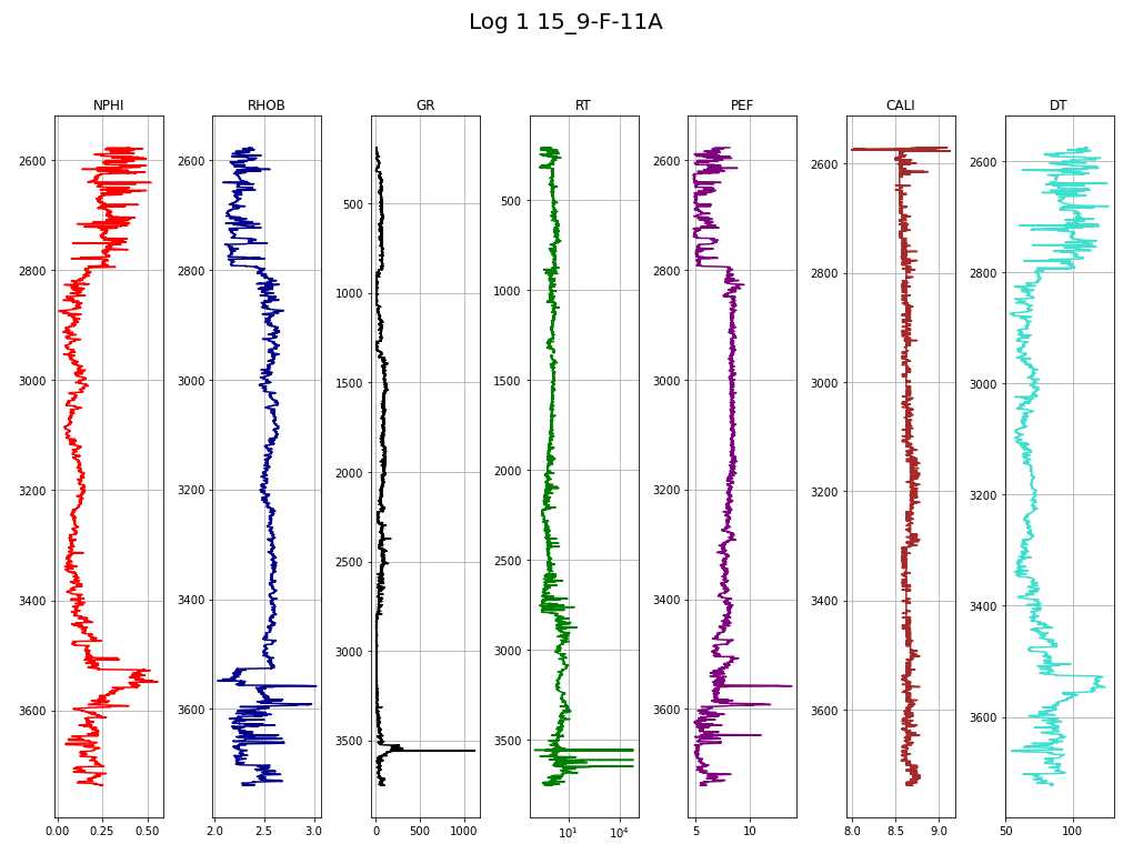
makeplot(log2, "Log 2 15_9-F-11B")
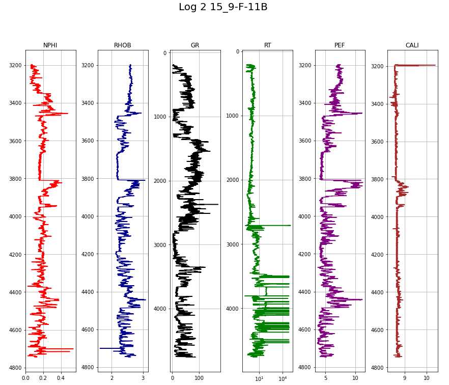
Data Preparation
# Lists of depths for clipping
lower = [2600, 3200, 2620, 3100, 3100]
upper = [3720, 4740, 3640, 3400, 4050]

# Lists of selected columns
train_cols = ['DEPTH', 'NPHI', 'RHOB', 'GR', 'RT', 'PEF', 'CALI', 'DT']
test_cols = ['DEPTH', 'NPHI', 'RHOB', 'GR', 'RT', 'PEF', 'CALI']

log_list_clipped = [0] * len(paths)

for i in range(len(log_list)):

  # Clip depths
  temp_df = log_list[i].loc[
      (log_list[i]['DEPTH'] >= lower[i]) &
      (log_list[i]['DEPTH'] <= upper[i])
  ]

  # Select train-log columns
  if i in [0,2,3]:
    log_list_clipped[i] = temp_df[train_cols]

  # Select test-log columns
  else:
    log_list_clipped[i] = temp_df[test_cols]

# Save logs from list into separate variables
log1, log2, log3, log4, log5 = log_list_clipped
# check for NaN
log1
DEPTH NPHI RHOB GR RT PEF CALI DT 24115 2600.0 0.371 2.356 82.748 1.323 7.126 8.648 104.605 24116 2600.1 0.341 2.338 79.399 1.196 6.654 8.578 103.827 24117 2600.2 0.308 2.315 74.248 1.171 6.105 8.578 102.740 24118 2600.3 0.283 2.291 68.542 1.142 5.613 8.547 100.943 24119 2600.4 0.272 2.269 60.314 1.107 5.281 8.523 98.473 … … … … … … … … … 35311 3719.6 0.236 2.617 70.191 1.627 7.438 8.703 84.800 35312 3719.7 0.238 2.595 75.393 1.513 7.258 8.750 85.013 35313 3719.8 0.236 2.571 82.648 1.420 7.076 8.766 85.054 35314 3719.9 0.217 2.544 89.157 1.349 6.956 8.781 84.928 35315 3720.0 0.226 2.520 90.898 1.301 6.920 8.781 84.784 # Concatenate dataframes
train = pd.concat([log1, log3, log4])
pred = pd.concat([log2, log5])
# Assign names
names = ['15_9-F-11A', '15_9-F-11B', '15_9-F-1A', '15_9-F-1B', '15_9-F-1C']
names_train = []
names_pred = []
for i in range(len(log_list_clipped)):
if i in [0,2,3]:
# Train data, assign names
names_train.append(np.full(len(log_list_clipped[i]), names[i]))
else:
# Test data, assign names
names_pred.append(np.full(len(log_list_clipped[i]), names[i]))
# Concatenate inside list
names_train = list(itertools.chain.from_iterable(names_train))
names_pred = list(itertools.chain.from_iterable(names_pred))
# Add well name to df
train['WELL'] = names_train
pred['WELL'] = names_pred
# Pop and add depth to end of df
depth_train, depth_pred = train.pop('DEPTH'), pred.pop('DEPTH')
train['DEPTH'], pred['DEPTH'] = depth_train, depth_pred
# Train dataframe with logs 1,3,4 vertically stacked
train
NPHI RHOB GR RT PEF CALI DT WELL DEPTH 24115 0.3710 2.3560 82.7480 1.3230 7.1260 8.6480 104.6050 15_9-F-11A 2600.0 24116 0.3410 2.3380 79.3990 1.1960 6.6540 8.5780 103.8270 15_9-F-11A 2600.1 24117 0.3080 2.3150 74.2480 1.1710 6.1050 8.5780 102.7400 15_9-F-11A 2600.2 24118 0.2830 2.2910 68.5420 1.1420 5.6130 8.5470 100.9430 15_9-F-11A 2600.3 24119 0.2720 2.2690 60.3140 1.1070 5.2810 8.5230 98.4730 15_9-F-11A 2600.4 … … … … … … … … … … 32537 0.1861 2.4571 60.4392 1.2337 5.9894 8.7227 75.3947 15_9-F-1B 3399.6 32538 0.1840 2.4596 61.8452 1.2452 6.0960 8.6976 75.3404 15_9-F-1B 3399.7 32539 0.1798 2.4637 61.1386 1.2960 6.1628 8.6976 75.3298 15_9-F-1B 3399.8 32540 0.1780 2.4714 59.3751 1.4060 6.1520 8.6976 75.3541 15_9-F-1B 3399.9 32541 0.1760 2.4809 58.3742 1.4529 6.1061 8.6978 75.4476 15_9-F-1B 3400.0 # Pred dataframe with logs 2, 5 verically stacked
pred
NPHI RHOB GR RT PEF CALI WELL DEPTH 30115 0.0750 2.6050 9.3480 8.3310 7.4510 8.5470 15_9-F-11B 3200.0 30116 0.0770 2.6020 9.3620 8.2890 7.4640 8.5470 15_9-F-11B 3200.1 30117 0.0780 2.5990 9.5450 8.2470 7.4050 8.5470 15_9-F-11B 3200.2 30118 0.0790 2.5940 11.1530 8.2060 7.2920 8.5470 15_9-F-11B 3200.3 30119 0.0780 2.5890 12.5920 8.1650 7.1670 8.5470 15_9-F-11B 3200.4 … … … … … … … … … 39037 0.3107 2.4184 106.7613 2.6950 6.2332 8.5569 15_9-F-1C 4049.6 39038 0.2997 2.4186 109.0336 2.6197 6.2539 8.5569 15_9-F-1C 4049.7 39039 0.2930 2.4232 106.0935 2.5948 6.2883 8.5570 15_9-F-1C 4049.8 39040 0.2892 2.4285 105.4931 2.6344 6.3400 8.6056 15_9-F-1C 4049.9 39041 0.2956 2.4309 109.8965 2.6459 6.3998 8.5569 15_9-F-1C 4050.0 Exploratory Data Analysis
Pair-plot of the Train Data
train_features = ['NPHI', 'RHOB', 'GR', 'RT', 'PEF', 'CALI', 'DT']

sns.pairplot(train, vars=train_features, diag_kind='kde',
             plot_kws = {'alpha': 0.6, 's': 30, 'edgecolor': 'k'})
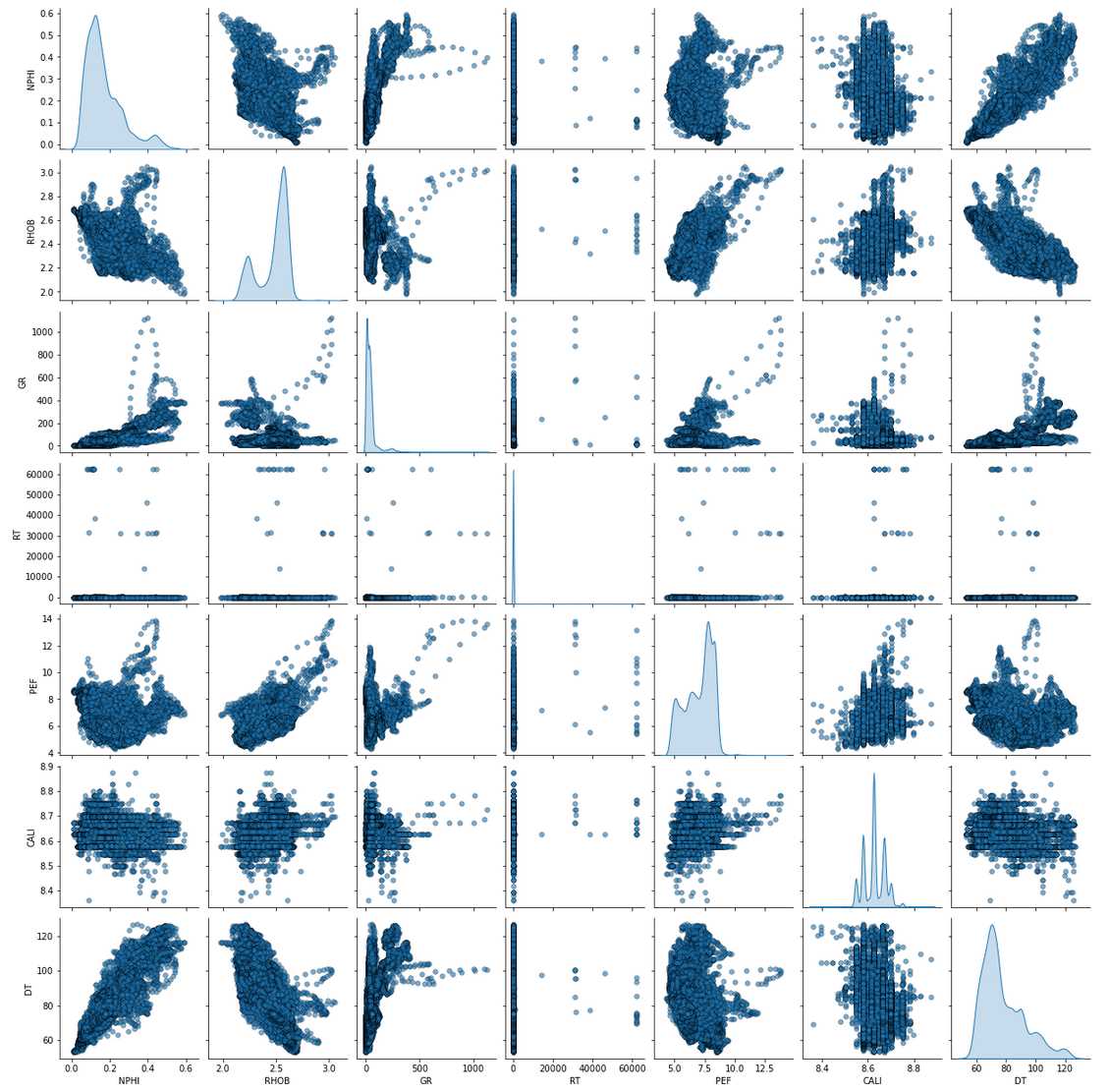
Spearman’s Correlation Heatmap
train_only_features = train[train_features]

# Generate a mask for the upper triangle
mask = np.zeros_like(train_only_features.corr(method = 'spearman') , dtype=np.bool)
mask[np.triu_indices_from(mask)] = True

# Custom colormap
cmap = sns.cubehelix_palette(n_colors=12, start=-2.25, rot=-1.3, as_cmap=True)

# Draw the heatmap with the mask and correct aspect ratio
plt.figure(figsize=(12,10))
sns.heatmap(train_only_features.corr(method = 'spearman'), annot=True,  mask=mask, cmap=cmap, vmax=.3, square=True)

plt.show()

Transformation of the Train Data
# Log transform the RT to logarithmic
train['RT'] = np.log10(train['RT'])

from sklearn.compose import ColumnTransformer
from sklearn.preprocessing import PowerTransformer

# Transformation / Normalizer object Yeo-Johnson method
scaler = PowerTransformer(method='yeo-johnson')

# ColumnTransformer (feature_target defines to which it is applied, leave Well and Depth untouched)
ct = ColumnTransformer([('transform', scaler, feature_target)], remainder='passthrough')

# Fit and transform
train_trans = ct.fit_transform(train)

# Convert to dataframe
train_trans = pd.DataFrame(train_trans, columns=colnames)
train_trans
NPHI RHOB GR RT PEF CALI DT WELL DEPTH 0 1.702168 -0.920748 1.130650 -0.631876 0.031083 0.450019 1.588380 15_9-F-11A 2600.0 1 1.573404 -1.020621 1.092435 -0.736154 -0.373325 -1.070848 1.562349 15_9-F-11A 2600.1 2 1.407108 -1.142493 1.030314 -0.758080 -0.819890 -1.070848 1.525055 15_9-F-11A 2600.2 3 1.260691 -1.263078 0.956135 -0.784153 -1.197992 -1.753641 1.460934 15_9-F-11A 2600.3 4 1.189869 -1.367969 0.837247 -0.816586 -1.441155 -2.286221 1.367432 15_9-F-11A 2600.4 … … … … … … … … … … 24398 0.462363 -0.279351 0.839177 -0.704005 -0.910619 2.041708 0.047941 15_9-F-1B 3399.6 24399 0.439808 -0.261621 0.860577 -0.694407 -0.826995 1.510434 0.043466 15_9-F-1B 3399.7 24400 0.393869 -0.232335 0.849885 -0.653120 -0.774093 1.510434 0.042591 15_9-F-1B 3399.8 24401 0.373838 -0.176628 0.822640 -0.569367 -0.782672 1.510434 0.044596 15_9-F-1B 3399.9 24402 0.351335 -0.106609 0.806807 -0.535769 -0.819021 1.514682 0.052292 15_9-F-1B 3400.0 Pair-Plot (after transformation)
sns.pairplot(train_trans, vars=feature_target, diag_kind = 'kde',
             plot_kws = {'alpha': 0.6, 's': 30, 'edgecolor': 'k'})
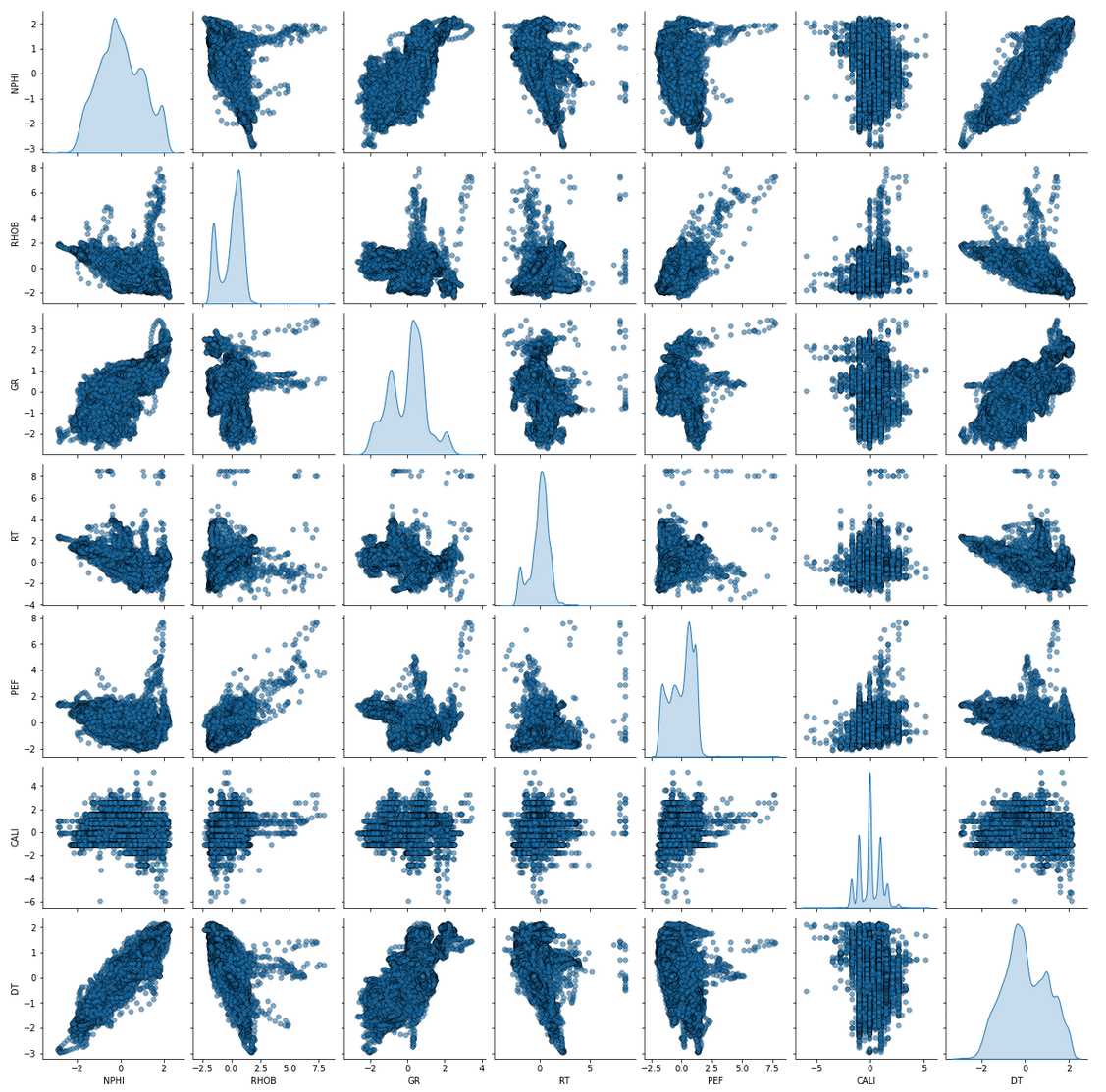
Removing Outliers
from sklearn.ensemble import IsolationForest
from sklearn.covariance import EllipticEnvelope
from sklearn.neighbors import LocalOutlierFactor
from sklearn.svm import OneClassSVM

# Make a copy of train
train_fonly = train_trans.copy()

# Remove WELL, DEPTH
train_fonly = train_fonly.drop(['WELL', 'DEPTH'], axis=1)
train_fonly_names = train_fonly.columns

# Helper function for repeated plotting

def makeboxplot(my_title='enter title',my_data=None):
    _, ax1 = plt.subplots()
    ax1.set_title(my_title, size=15)
    ax1.boxplot(my_data)
    ax1.set_xticklabels(train_fonly_names)
    plt.show()

makeboxplot('Unprocessed',train_trans[train_fonly_names])
print('n samples unprocessed:', len(train_fonly))
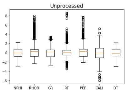
Method 1: Standard Deviation
train_stdev = train_fonly[np.abs(train_fonly - train_fonly.mean()) <= (3 * train_fonly.std())]

# Delete NaN
train_stdev = train_stdev.dropna()

makeboxplot('Method 1: Standard Deviation',train_stdev)
print('Remaining samples:', len(train_stdev))
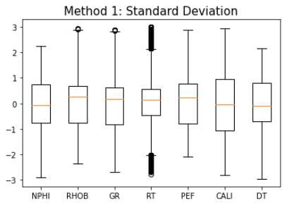
Method 2: Isolation Forest
iso = IsolationForest(contamination=0.5)
yhat = iso.fit_predict(train_fonly)
mask = yhat != -1
train_iso = train_fonly[mask]

makeboxplot('Method 2: Isolation Forest',train_iso)
print('Remaining Samples:', len(train_iso))
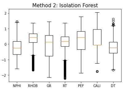
Method 3: Minimum Covariance Determinant
ee = EllipticEnvelope(contamination=0.1)
yhat = ee.fit_predict(train_fonly)
mask = yhat != -1
train_ee = train_fonly[mask]

makeboxplot('Method 3: Minimum Covariance Determinant',train_ee)
print('Remaining samples:', len(train_ee))
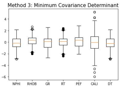
Method 4: Local Outlier Factor
lof = LocalOutlierFactor(contamination=0.3)
yhat = lof.fit_predict(train_fonly)
mask = yhat != -1
train_lof = train_fonly[mask]

makeboxplot('Method 4: Local Outlier Factor',train_lof)
print('Remaining samples:', len(train_lof))
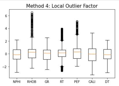
Method 5: Support Vector Machine
svm = OneClassSVM(nu=0.1)
yhat = svm.fit_predict(train_fonly)
mask = yhat != -1
train_svm = train_fonly[mask]

makeboxplot('Method 5: Support Vector Machine',train_svm)
print('Remaining samples:', len(train_svm))
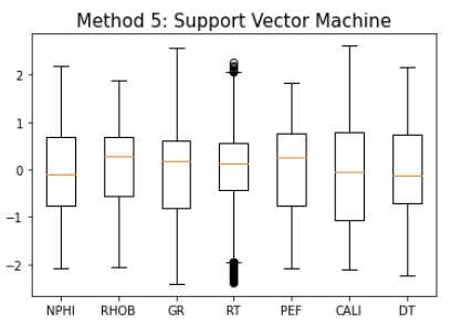
sns.pairplot(train_svm, vars=feature_target,
             diag_kind='kde',
             plot_kws = {'alpha': 0.6, 's': 30, 'edgecolor': 'k'})
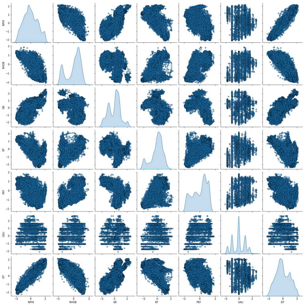
Train and Validate
# Select columns for features (X) and target (y)
X_train = train_svm[feature_names].values
y_train = train_svm[target_name].values

Define the validation data
train_trans_copy = train_trans.copy()

train_well_names = ['15_9-F-11A', '15_9-F-1A', '15_9-F-1B']

X_val = []
y_val = []

for i in range(len(train_well_names)):
  # Split the df by log name
  val = train_trans_copy.loc[train_trans_copy['WELL'] == train_well_names[i]]

  # Drop name column
  val = val.drop(['WELL'], axis=1)

  # Define X_val (feature) and y_val (target)
  X_val_, y_val_ = val[feature_names].values, val[target_name].values

  X_val.append(X_val_)
  y_val.append(y_val_)

# save into separate dfs
X_val1, X_val3, X_val4 = X_val
y_val1, y_val3, y_val4 = y_val
Fit to Test and Score on Val
from sklearn.metrics import mean_squared_error
from sklearn.ensemble import GradientBoostingRegressor

# Gradient Booster object
model = GradientBoostingRegressor()

# Fit the regressor to the training data
model.fit(X_train, y_train)

# Validation: Predict on well 1
y_pred1 = model.predict(X_val1)
print("R2 Log 1: {}".format(round(model.score(X_val1, y_val1),4)))
rmse = np.sqrt(mean_squared_error(y_val1, y_pred1))
print("RMSE Log 1: {}".format(round(rmse,4)))

# Validation: Predict on well 3
y_pred3 = model.predict(X_val3)
print("R2 Log 3: {}".format(round(model.score(X_val3, y_val3),4)))
rmse = np.sqrt(mean_squared_error(y_val3, y_pred3))
print("RMSE Log 3: {}".format(round(rmse,4)))

# Validation: Predict on well 4
y_pred4 = model.predict(X_val4)
print("R2 Log 4: {}".format(round(model.score(X_val4, y_val4),4)))
rmse = np.sqrt(mean_squared_error(y_val4, y_pred4))
print("RMSE Log 4: {}".format(round(rmse,4)))
Inverse Transformation of Prediction
# Make the transformer fit to the target
y = train[target_name].values
scaler.fit(y.reshape(-1,1))

# Inverse transform  y_val, y_pred
y_val1, y_pred1 = scaler.inverse_transform(y_val1.reshape(-1,1)), scaler.inverse_transform(y_pred1.reshape(-1,1))
y_val3, y_pred3 = scaler.inverse_transform(y_val3.reshape(-1,1)), scaler.inverse_transform(y_pred3.reshape(-1,1))
y_val4, y_pred4 = scaler.inverse_transform(y_val4.reshape(-1,1)), scaler.inverse_transform(y_pred4.reshape(-1,1))
x = [y_val1, y_pred1, y_val3, y_pred3, y_val4, y_pred4]
y = [log1['DEPTH'], log1['DEPTH'], log3['DEPTH'], log3['DEPTH'], log4['DEPTH'], log4['DEPTH']]

color = ['red', 'blue', 'red', 'blue', 'red', 'blue']
title = ['DT Log1 1', 'Pred. DT Log 1', 'DT Log 3', 'Pred DT Log 3',
         'DT Log 4', 'Pred DT Log 4']

fig, ax = plt.subplots(nrows=1, ncols=6, figsize=(15,10))

for i in range(len(x)):
  ax[i].plot(x[i], y[i], color=color[i])
  ax[i].set_xlim(50, 150)
  ax[i].set_ylim(np.max(y[i]), np.min(y[i]))
  ax[i].set_title(title[i])

plt.tight_layout()

plt.show()
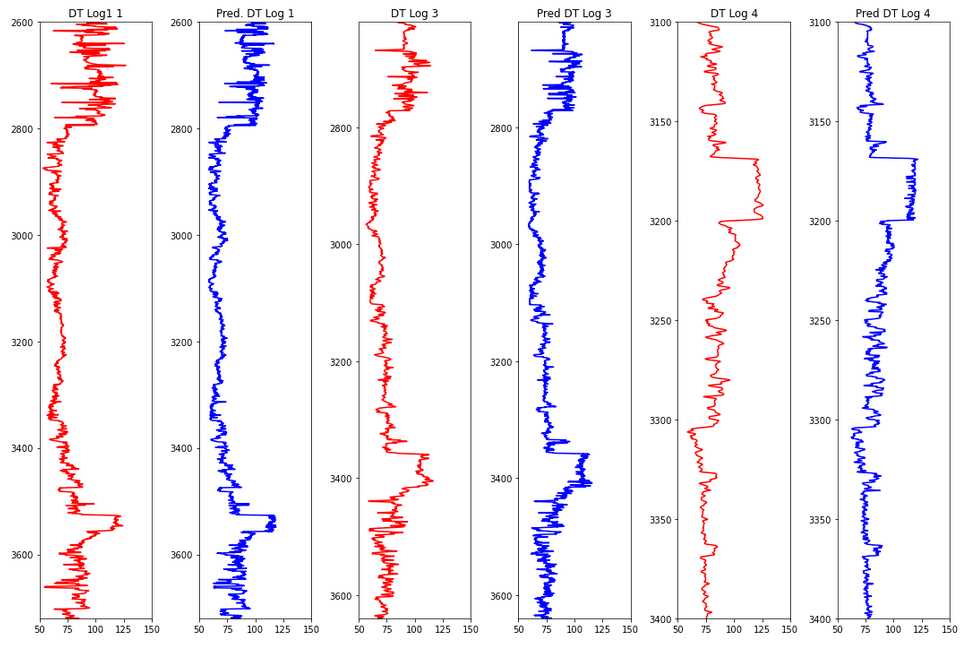
Hyperparameter Tuning
GridSearchCV hyperparameter tuning on Scikit-Learn’s GradientBoostingRegressor, resulting in 31 models playing through all variations.from sklearn.model_selection import train_test_split
# Define the X and y from the SVM normalized dataset
X = train_svm[feature_names].values
y = train_svm[target_name].values
# Train and test split
X_train, X_test, y_train, y_test = train_test_split(X, y, test_size=0.3, random_state=42)
from sklearn.model_selection import GridSearchCV

model = GradientBoostingRegressor()

# Hyperparameter ranges

max_features = ['auto', 'sqrt']
min_samples_leaf = [1, 4]
min_samples_split = [2, 10]
max_depth = [10, 100]
n_estimators = [100, 1000]

param_grid = {'max_features': max_features,
              'min_samples_leaf': min_samples_leaf,
              'min_samples_split': min_samples_split,
              'max_depth': max_depth,
              'n_estimators': n_estimators}

# Train with grid
model_random = GridSearchCV(model, param_grid, cv=3)
model_random.fit(X_train, y_train)

# Print best model
model_random.best_params_
Predict Test Wells
Define the Test Data
# Define the test data
names_test = ['15_9-F-11B', '15_9-F-1C']

X_test = []
y_test = []
depths = []

for i in range(len(names_test)):
  # split the df with respect to its name
  test = pred.loc[pred['WELL'] == names_test[i]]

  # Drop well name column
  test = test.drop(['WELL'], axis=1)

  # Define X_test (feature)
  X_test_ = test[feature_names].values

  # Define depth
  depth_ = test['DEPTH'].values

  X_test.append(X_test_)
  depths.append(depth_)

# For each well 2 and 5
X_test2, X_test5 = X_test
depth2, depth5 = depths
Transform Test - Predict - Inverse Transform
# Transform X_test of log 2 and 5
X_test2 = scaler.fit_transform(X_test2)
X_test5 = scaler.fit_transform(X_test5)

# Predict to log 2 and 5 with tuned model
y_pred2 = model_random.predict(X_test2)
y_pred5 = model_random.predict(X_test5)

y = train[target_name].values
scaler.fit(y.reshape(-1,1))

# Inverse transform y_pred
y_pred2 = scaler.inverse_transform(y_pred2.reshape(-1,1))
y_pred5 = scaler.inverse_transform(y_pred5.reshape(-1,1))
Plot the Predictions
plt.figure(figsize=(5,12))

plt.subplot(1,2,1)
plt.plot(y_pred2, depth2, color='green')
plt.ylim(max(depth2), min(depth2))
plt.title('Pred DT Log 2: 15_9-F-11B', size=12)

plt.subplot(1,2,2)
plt.plot(y_pred5, depth5, color='green')
plt.ylim(max(depth5), min(depth5))
plt.title('Pred DT Log 5: 15_9-F-1C', size=12)

plt.tight_layout()
plt.show()
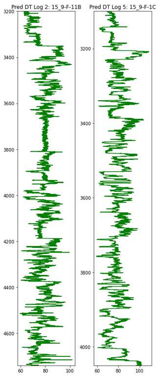
def makeplotpred(df,suptitle_str="pass a suptitle"):
  # Column selection from df
  col_names = ['NPHI', 'RHOB', 'GR', 'RT', 'PEF', 'CALI', 'DT']
  # Plotting titles
  title = ['NPHI', 'RHOB', 'GR', 'RT', 'PEF', 'CALI', 'Predicted DT']
  # plotting colors
  colors = ['purple', 'purple', 'purple', 'purple', 'purple', 'purple', 'green']

  # Create the subplots; ncols equals the number of logs
  fig, ax = plt.subplots(nrows=1, ncols=len(col_names), figsize=(15,10))
  fig.suptitle(suptitle_str, size=20, y=1.05)

  # Looping each log to display in the subplots
  for i in range(len(col_names)):
    if i == 3:
      # for resistivity, semilog plot
      ax[i].semilogx(df[col_names[i]], df['DEPTH'], color=colors[i])
    else:
      # for non-resistivity, normal plot
      ax[i].plot(df[col_names[i]], df['DEPTH'], color=colors[i])

    ax[i].set_ylim(max(df['DEPTH']), min(df['DEPTH']))
    ax[i].set_title(title[i], pad=15)
    ax[i].grid(True)

  ax[2].set_xlim(0, 200)
  plt.tight_layout(1)
  plt.show()
makeplotpred(log2,"Log 2: 15_9-F-11B")
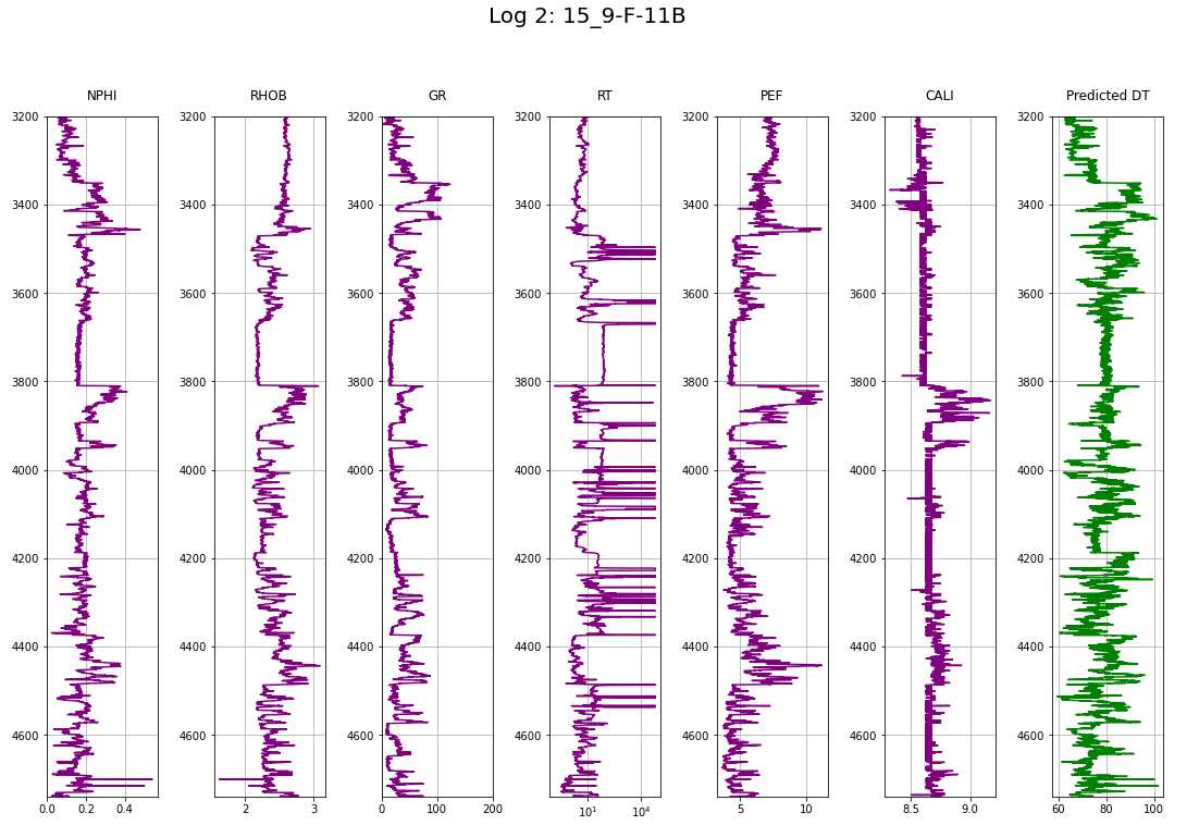
makeplotpred(log5,"Log 5: 15_9-F-1C")
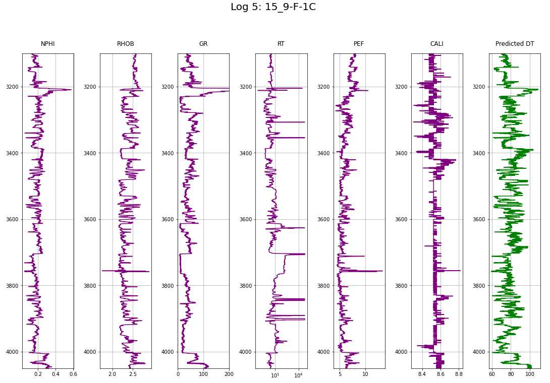
ADV SQL QRIES

CASE
CASE WHEN THEN ELSE END AS. The ELSE and AS are optionalSELECT
m.date,
t.team_long_name AS opponent,
CASE WHEN m.home_goal < m.away_goal THEN 'Barcelona win!'
WHEN m.home_goal > m.away_goal THEN 'Barcelona loss :('
ELSE 'Tie' END AS outcome
FROM matches_spain AS m
LEFT JOIN teams_spain AS t
ON m.hometeam_id = t.team_api_id
WHERE m.awayteam_id = 8634;
CASE and aggregate function (SUM)
SELECT
	c.name AS country,
	SUM(CASE WHEN m.season = '2012/2013' AND m.home_goal > m.away_goal
			 THEN 1 ELSE 0 END) AS matches_2012_2013,

	SUM(CASE WHEN m.season = '2013/2014' AND m.home_goal > m.away_goal
			 THEN 1 ELSE 0 END) AS matches_2013_2014,

	SUM(CASE WHEN m.season = '2014/2015' AND m.home_goal > m.away_goal
			 THEN 1 ELSE 0 END) AS matches_2014_2015
FROM country AS c
LEFT JOIN match AS m
ON c.id = m.country_id
GROUP BY country;
Percentages with AVG and CASE
AVG and CASE (for 1,0 assignment) functions.SELECT
c.name AS country,
ROUND(AVG(CASE WHEN m.season='2013/2014' AND m.home_goal = m.away_goal THEN 1
WHEN m.season='2013/2014' AND m.home_goal != m.away_goal THEN 0
END),2) AS pct_ties_2013_2014,
ROUND(AVG(CASE WHEN m.season='2014/2015' AND m.home_goal = m.away_goal THEN 1
WHEN m.season='2014/2015' AND m.home_goal != m.away_goal THEN 0
END),2) AS pct_ties_2014_2015
FROM country AS c
LEFT JOIN matches AS m
ON c.id = m.country_id
GROUP BY country;
TRY queries and CATCH errors
BEGIN TRY
	ALTER TABLE products
		ADD CONSTRAINT CHK_Stock CHECK (stock >= 0);
END TRY

BEGIN CATCH
	SELECT 'There was an error adding the constraing!';
END CATCH
Nested TRY/CATCH
BEGIN TRY
	INSERT INTO bikes (make, model, year, size)
		VALUES ('Nukeproof', 'Grizzlybear', '2021', 'S');
END TRY

BEGIN CATCH
	SELECT 'An error occurred inserting the bike!';
    BEGIN TRY
    	INSERT INTO errors
        	VALUES ('Error inserting a bike');
        SELECT 'Error inserted correctly!';
	END TRY

    BEGIN CATCH
    	SELECT 'An error occurred inserting the error!';
    END CATCH
END CATCH
CATCH Error Details
BEGIN TRY
	INSERT INTO bikes (make, model, year, size)
		VALUES ('Nukeproof', 'Grizzlybear', '2021', 'S');
END TRY

BEGIN CATCH
	SELECT 'An error occurred inserting the product!';
    BEGIN TRY
    	INSERT INTO errors
        	VALUES ('Error inserting a product');
    END TRY

    BEGIN CATCH
    	SELECT  ERROR_NUMBER() AS number,
        	ERROR_SEVERITY() AS severity_level,
        	ERROR_STATE() AS state,
        	ERROR_LINE() AS line,
        	ERROR_MESSAGE() AS message;
    END CATCH
END CATCH
Custom Errors, RAISERROR
RAISERROR ( { msg_str | msg_id | @local_variable_message },
    severity,
    state,
    [ argument [ ,...n ] ] )
    [ WITH option [ ,...n ] ]
@product_id = 56747

BEGIN TRY
IF NOT EXISTS (SELECT * FROM products WHERE product_id = @product_id)
	RAISERROR('No product with id %d.', 11, 1, @product_id);
ELSE
	SELECT * FROM products WHERE product_id = @product_id;
END TRY

BEGIN CATCH
    SELECT  ERROR_NUMBER() AS number,
        ERROR_SEVERITY() AS severity_level,
        ERROR_STATE() AS state,
        ERROR_LINE() AS line,
        ERROR_MESSAGE() AS message;
END CATCH
Subqueries
Subqueries in WHERE clause
SELECT
	team_long_name,
	team_short_name
FROM team
WHERE team_api_id IN
	(SELECT hometeam_id
	 FROM match
	 WHERE home_goal >= 8);
Subqueries in FROM
SELECT
	country,
	date,
	home_goal,
	away_goal
FROM
	(SELECT c.name AS country,
			m.date,
			m.home_goal,
			m.away_goal,
			(m.home_goal + m.away_goal) AS total_goals
	FROM match AS m
	LEFT JOIN country AS c
	ON m.country_id = c.id) AS subq
WHERE total_goals >= 10;
Subqueries in SELECT
SELECT statements generate a single value!SELECT
l.name AS league,
ROUND(AVG(m.home_goal + m.away_goal), 2) AS avg_goals
(SELECT ROUND(AVG(home_goal + away_goal), 2)
FROM match
WHERE season = '2013/2014') AS overall_avg
FROM league AS l
LEFT JOIN match AS m
ON l.country_id = m.country_id
WHERE season = '2013/2014'
GROUP BY league;
Correlated Subqueries
WHERE clause filters for entries with total goals higher than three times the average.SELECT
main.country_id,
date,
main.home_goal,
main.away_goal
FROM match AS main
WHERE
(home_goal + away_goal) >
(SELECT AVG((sub.home_goal + sub.away_goal) * 3)
FROM match AS sub
WHERE main.country_id = sub.country_id);
Nested Subqueries in FROM
SELECT
	c.name AS country,
	AVG(outer_s.matches) AS avg_seasonal_high_scores
FROM country AS c
LEFT JOIN (
		SELECT country_id, season,
			COUNT(id) AS matches
		FROM (
			SELECT country_id, season, id
			FROM match
			WHERE home_goal >= 5 OR away_goal >= 5) AS inner_s
		GROUP BY country_id, season) AS outer_s
ON c.id = outer_s.country_id
GROUP BY country;
Common Table Expressions (CTE)
WITH cte AS (SELECT…..)WITH home AS (
SELECT m.id,
m.date,
t.team_long_name AS hometeam,
m.home_goal
FROM match AS m
LEFT JOIN team AS t
ON m.hometeam_id = t.team_api_id),
away AS (
SELECT m.id,
m.date,
t.team_long_name AS awayteam,
m.away_goal
FROM match AS m
LEFT JOIN team AS t
ON m.awayteam_id = t.team_api_id)
SELECT
home.date,
home.hometeam,
away.awayteam,
home.home_goal,
away.away_goal
FROM home
INNER JOIN away
ON home.id = away.id;
Window Functions - They all use OVER()
OVER() clause allows you to pass an aggregate function down a data set, similar to subqueries in SELECT, but run faster.OVER() generates column with an aggregate of the complete column and the same value in each row.SELECT
m.id,
c.name AS country,
m.season,
m.home_goal,
m.away_goal,
AVG(m.home_goal + m.away_goal) OVER() AS overall_avg
FROM match AS m
LEFT JOIN country AS c ON m.country_id = c.id;
OVER(ORDER BY...) calculates the running total/sum up to the current row.SELECT
athlete,
medals,
SUM(medals) OVER(ORDER BY athlete ASC) AS sum_medals
FROM athlete_medals
ORDER BY athlete ASC;
RANK()
SELECT
	l.name AS league,
	AVG(m.home_goal + m.away_goal) AS avg_goals,
	RANK() OVER(ORDER BY AVG(m.home_goal + m.away_goal) DESC) AS league_rank
FROM league AS l
LEFT JOIN match AS m
ON l.id = m.country_id
WHERE m.season = '2011/2012'
GROUP BY l.name
ORDER BY league_rank;
SELECT
  athlete,
  medals,
  RANK() OVER (ORDER BY medals DESC) AS Rank_N
FROM Athlete_Medals
ORDER BY Medals DESC;
DENSE_RANK()
SELECT
  country,
  athlete,
  DENSE_RANK() OVER (PARTITION BY country ORDER BY medals DESC) AS rank_n
FROM athlete_medals
ORDER BY country ASC, rank_n ASC;
Giving rows a number with ROW_NUMBER()
ROW_NUMBER().SELECT
*,
ROW_NUMBER() OVER() AS Row_N
FROM Summer_Medals
ORDER BY Row_N AS
ORDER BY inside the OVER() clause takes precedence over outer ORDER BY. The following queries only calls distinct years and does not requrie a subquery.SELECT
Year,
ROW_NUMBER() OVER(ORDER BY Year ASC) AS Row_N
FROM (
SELECT DISTINCT Year
FROM Summer_Medals
) AS Yea
Framing for sliding windows using RANGE BETWEEN…AND or ROWS BETWEEN…AND
UNBOUNDED, n PRECEDING, n FOLLOWING, and CURRENT ROWRANGE vs. ROW: RANGE() treats duplicates in OVER(ORDER BY...) as a single entity, which is a special case. ROWS behaves normally.Medals Rows Running Total Range Running Total 10 10 10 50 60 110 50 110 110 60 170 230 60 230 230 70 300 300 SELECT
date,
home_goal,
away_goal,
SUM(home_goal) OVER(ORDER BY date
ROWS BETWEEN UNBOUNDED PRECEDING AND CURRENT ROW) AS running_total,
AVG(home_goal) OVER(ORDER BY date
ROWS BETWEEN UNBOUNDED PRECEDING AND CURRENT ROW) AS running_avg
FROM match
WHERE
hometeam_id = 9908
AND season = '2011/2012';
SELECT
	date,
	home_goal,
	away_goal,
	SUM(home_goal) OVER(ORDER BY date DESC
		ROWS BETWEEN CURRENT ROW AND UNBOUNDED FOLLOWING) AS running_total,
	AVG(home_goal) OVER(ORDER BY date DESC
		ROWS BETWEEN CURRENT ROW AND UNBOUNDED FOLLOWING) AS running_avg
FROM match
WHERE
	awayteam_id = 9908
    AND season = '2011/2012';
SELECT
	year,
	medals,
	AVG(medals) OVER(ORDER BY year ASC
		ROWS BETWEEN 2 PRECEDING AND CURRENT ROW) AS medals_ma
FROM russian_medals
ORDER BY year ASC;
Fetching relative rows: LAG() and LEAD()
LAG(column, n) function fetches a single value from BEFORE (above) the current row (given vertical lag distance) for creating a new column.SELECT
Year, Champion,
LAG(Champion) OVER(ORDER BY year ASC) AS Last_Champion
FROM weightlifting_gold
ORDER BY year ASC;
LEAD(column, n) function fetches a single value from AFTER (below) the current row (given vertical lag distance) for creating a new column.SELECT
year,
athlete,
LEAD(athlete, 3) OVER (ORDER BY year ASC) AS future_champion
FROM discus_medalists
ORDER BY year ASC;
Fetching absolute rows: FIRST_VALUE() and LAST_VALUE()
FIRST_VALUE(column) and LAST_VALUE(column)SELECT
athlete,
FIRST_VALUE(athlete) OVER(ORDER BY athlete ASC) AS First_Athlete
FROM all_male_medalists;
RANGE BETWEEN UNBOUNDED PRECEDING AND UNBOUNDED FOLLOWING.SELECT
year,
city,
LAST_VALUE(city) OVER(ORDER BY year ASC
RANGE BETWEEN
UNBOUNDED PRECEDING AND
UNBOUNDED FOLLOWING
) AS last_city
FROM hosts
ORDER BY Year ASC;
PARTITION BY subdivides processing ranges in a column
ROW_NUMBER or LAG() functions.LAG() function determining gold winners of ‘male’ spilling into ‘females’. In that case, a null value will be displayed.SELECT
gender,
year,
country AS champion,
LAG(country,1) OVER(PARTITION BY gender ORDER BY year ASC) AS last_champion
FROM athletics_gold
ORDER BY gender ASC, year ASC;
SELECT
	gender,
	year,
	event,
	country AS champion,
	LAG(country,1) OVER (PARTITION BY gender, event ORDER BY year ASC) AS last_champion
FROM athletics_gold
ORDER BY event ASC, gender ASC, year ASC;
Paging with NTILE()- subdivide a table into equal-length pages
NTILE(num_pages) OVER(ORDER BY column) AS new_column divides the table into num_pages depending on how the values in the given column. The new column contains the number of which page they were assigned. These pages are practically quantiles on which statistical analysis can be performed.SELECT
athlete,
medals,
NTILE(3) OVER(ORDER BY medals DESC) AS third
FROM athlete_medals
ORDER BY medals DESC, athlete ASC;
WITH thirds AS (
	SELECT
		athlete,
		medals,
		NTILE(3) OVER(ORDER BY medals DESC) AS third
	FROM athlete_medals)

SELECT
	third,
	AVG(medals) AS avg_medals
FROM thirds
GROUP BY third
ORDER BY third ASC;
Pivoting with the CROSSTAB() Extension
CROSSTAB requires the tablefunc extension that needs to be created befor qerrying.SELECT * FROM CROSSTAB($$....) AS ct (column COLTYPE,...) function and the new pivoted column names defined.CREATE EXTENSION IF NOT EXISTS tablefunc;
SELECT * FROM CROSSTAB($$
SELECT
gender,
year,
country
FROM summer_medals
WHERE
year IN (2008, 2012)
AND medal = 'gold'
AND event = 'pole vault'
ORDER BY gender ASC, year ASC;
$$) AS ct (gender VARCHAR,
"2008" VARCHAR,
"2012" VARCHAR)
ORDER BY gender ASC;
gender year country Men 2008 AUS Men 2012 FRA Women 2008 RUS Women 2012 USA gender 2008 2012 Men AUS FRA Women RUS USA Group total rows with GROUP BY ROLLUP() and CUBE()
Null entries in the rows signifies the total rows.ROLLUP(gender) clause.SELECT
country,
gender,
COUNT(*) AS gold_awards
FROM summer_medals
WHERE
year = 2004
AND medal = 'Gold'
AND country IN ('DEN', 'NOR', 'SWE')
GROUP BY country, ROLLUP(gender)
ORDER BY country ASC, gender ASC;
CUBE(). Note: all columns have to go into the CUBE() or it will fail.SELECT
gender,
medal,
COUNT(*) AS awards
FROM Summer_Medals
WHERE
year = 2012
AND country = 'RUS'
GROUP BY CUBE(gender, medal)
ORDER BY gender ASC, medal ASC;
Fill Null values with COALESCE()
ROLLUP(), CUBE(), pivoting, first/last row of LAG(), LEAD().SELECT section of query: COALESCE(column, 'null filler string') AS column.SELECT
COALESCE(country, 'all countries') AS country,
COALESCE(gender, 'all genders') AS gender,
COUNT(*) AS awards
FROM summer_medals
WHERE
year = 2004
AND medal = 'gold'
AND country IN ('DEN', 'NOR', 'SWE')
GROUP BY ROLLUP(country, cender)
ORDER BY country ASC, gender ASC;
String Manipulation
Compress a Column into a single String with STRING_AGG()
SELECT statemtt like as such: STRING_AGG(column, 'separator')SELECT
STRING_AGG(country, ', ')
FROM country_ranks
WHERE rank_col <= 3;
Country Rank USA 1 RUS 2 AUS 3 … … Concatenating Multiple Columns with || and CONCAT()
SELECT
	first_name || ' ' || last_name AS full_name
FROM
	film;
SELECT
	customerID || ': ' || first_name || ' ' || last_name AS full_name;
CONCAT()SELECT
CONCAT(first_name,' ', last_name) AS full_name
FROM
film;
Changing Case with UPPER(), LOWER(), INITCAP()
SELECT
	UPPER(email)
FROM customer;
SELECT
	LOWER(email)
FROM customer;
SELECT
	INITCAP(title)
FROM film;
Replace Characters with REPLACE()
SELECT
	REPLACE(email, 'hedgeAThog.com', '[email protected]') AS email
FROM customer;
Trim Characters with TRIM(), LTRIM(), RTRIM()
TRIM([leading | trailing | both][characters] from string)space chars is be removed by default.space char is the default.SELECT
TRIM(),
LTRIM(' [email protected] '),
RTRIM(' [email protected] ')
Pad Characters with PAD(), LPAD(), RPAD()
LPAD(input_string, length_after_pad, lpad_string) Note that if the input string is shorter than the padded length, then no padding string will be inserted! If no padding string passed, is entered, then space char is the default.SELECT
LPAD('[email protected]', 20, '#'),
RPAD('[email protected]', 17, '$')
Reverse char order with REVERSE()
SELECT
	email,
	REVERSE(email)
FROM customer;
Character Count with CHAR_LENGTH() or LENGTH()
SELECT
	title,
	CHAR_LENGTH(title)
	LENGTH(title)
FROM film;
Find Char Position with STRPOS() or POSITION()
SELECT
	email,
	STRPOS(email, '@'),
	POSITION('@' IN email)
FROM customer;
Clip Strings from the Ends with LEFT(), RIGHT(), and SUBSTRING()
SELECT
	RIGHT(column_name, 50),
	LEFT(column_name, 10)
FROM customer;
SELECT
	SUBSTRING(column_name, 10, 50),
	SUBSTR(colum_name, 10, 50)
FROM customer;
SELECT
	SUBSTRING(email FROM 0 FOR POSITION('@' IN email)), -- name part of address up to @
	SUBSTRING(email FROM POSITION('@' IN email)+1 FOR CHAR_LENGTH(email)) -- provider part of address starting after @
FROM customer;
SELECT
	LEFT(description, 50 - POSITION(' ' IN REVERSE(LEFT(description, 50)) -- Subtract the position of the first whitespace character
FROM film;
Data Types
Casting Data Types
column :: data-typeSELECT
NOW():: timestamp;
CAST(column AS data-type) function.SELECT
CAST(NOW() AS timestamp);
Creating Data Types (PostgreSQL)
CREATE
	TYPE dayofweek as ENUM(
		'Monday',
		'Tuesday',
		'Wednesday',
		'Thursday',
		'Friday',
		'Saturday',
		'Sunday'
		);
Getting Information about Data Types (PostgreSQL)
SELECT
	typname,
	typcategory
FROM pg_type
WHERE typname = 'dayofweek';
User-Defined Functions (PostgreSQL)
CREATE.CREATE FUNCTION squared (i integer) RETURNS integer AS $$
BEGIN
RETURN i*i;
END;
$$ language plpgsql; --define language
SELECT
squared(10);
Text Search and NLP (PostgreSQL)
Full-Text Search (PostgreSQL)
WHERE column LIKE '%mystring%' with wildcards (%,_) etc. capabilities.SELECT
title,
description
FROM film
WHERE to_tsvector(title) @@ to_tsquery('elf');
Compare Two Strings (PostgreSQL)
SELECT
	levenshtein('hugo', 'hagolm');
similarity('hugo', 'hagolm');
Drop Duplicate Rows (based on Specific Columns)
WITH cte AS (
    SELECT *,
        ROW_NUMBER() OVER (
            PARTITION BY
                col_1,
                col_2,
                col_3
			ORDER BY
                col_1,
                col_2,
                col_3
        ) row_num
    FROM orders_table
)
SELECT *
FROM cte
WHERE row_num = 1;
id sales worker_firstname worker_lastname registration_date row_num 000000119 13 Johnny Smith 2014-01-31 1 000000127 14 Brian Merkel 2014-02-28 1 000000120 29 Karin Harris 2014-01-31 1 000000128 16 Carol Schulze 2014-02-28 1 Time Manipulation
NOW() and CURRENT_TIMESTAMP() fetch time (millisecond precision) with timezone! However, CURRENT_TIMESTAMP(2) can be passed an argument for roundeding to digits. If the timezone is not required, then these two functions can be cast to timestamp data-type.CURRENT_DATE only fetches the date portion of the CURRENT_TIMESTAMP()CURRENT_TIME() only fetches the time portion (with timezone) of the CURRENT_TIMESTAMP(). Can be passed rounding parameter.Intervals and Time Differences
INTERVAL function. The INTERVAL add 3 days to the rental date so we can compare if the return date was in time.SELECT
rental_date,
return_date,
rental_date + INTERVAL '+ `+3 days' AS expected_return_date
FROM rental;
SELECT
	title,
	INTERVAL '1' day * f.rental_duration AS rental_duration,
	return_date - rental_date AS days_rented
FROM film
WHERE return_date IS NOT NULL
AGE() function calculates an INTERVAL between a given timestamp/date and NOW if ONE parameter given. If TWO parameters are given, then the interval between those.SELECT
AGE(rental_date)
FROM rental;
Extracting from Timestamps
EXTRACT(field FROM source) and DATE_PART('field',source), which produce interchangeable results.Field (long) Field (short) Description year y Year quarter Quarter month Month day d Day of Month dow Day of Week week w Week hour h hour minute m Minute second s Second millisecond ms Millisecond SELECT
EXTRACT(quarter FROM TIMESTAMP '2009-02-12 05:18:00') AS quarter;
SELECT
	DATE_PART('quarter', TIMESTAMP '2009-02-12 05:18:00') AS quarter;
SELECT
	EXTRACT(dow FROM rental_date) AS dayofweek,
	COUNT(*) as rentals
FROM rental
GROUP BY 1; -- column called by positional index instead of names
SELECT
	EXTRACT(quarter FROM payment_date) AS quarter,
	EXTRACT(year FROM payment_date) AS year,
	SUM(amount) AS total_payments
FROM payment
GROUP BY 1, 2;
SELECT
	EXTRACT(dow FROM r.rental_date) AS dayofweek,
	AGE(return_date, rental_date) AS rental_days
FROM rental AS r
WHERE rental_date
	BETWEEN CAST('2005-05-01' AS TIMESTAMP)
	AND CAST('2005-05-01' AS TIMESTAMP) + INTERVAL '90 day';
Truncating Timestamps
DATE_TRUNC() function will truncate a timmestamp or interval data types from fine detail (e.g., minutes) to low detail (e.g., year). This means the timestamp’s length remains the same but set to the lowest logical value (01 for days/months, 00 for hours/minutes/seconds).SELECT
DATE_TRUNC('year', TIMESTAMP '2009-02-12 05:18:00';
SELECT
	DATE_TRUNC('month', TIMESTAMP '2009-02-12 05:18:00';
SELECT
	DATE_TRUNC('day', rental_date) AS rental_day,
	COUNT(*) AS rentals
FROM rental
GROUP BY 1;
Transactions (MS SQL SERVER)
With TRY/CATCH
BEGIN TRY
	BEGIN TRAN;
		UPDATE accounts SET current_balance = current_balance - 100 WHERE account_id = 4451;
		INSERT INTO transactions VALUES (4451, -100, GETDATE());

		UPDATE accounts SET current_balance = current_balance + 100 WHERE account_id = 6743;
		INSERT INTO transactions VALUES (4451, 100, GETDATE());
	COMMIT TRAN;
END TRY

BEGIN CATCH
	SELECT 'Rolling back the transaction';
	ROLLBACK TRAN;
END CATCH
With XACT_ABORT
SET XACT_ABORT ON;

BEGIN TRAN;
	UPDATE accounts set current_balance = current_balance - current_balance * 0.01 / 100
		WHERE current_balance > 5000000;
	IF @@ROWCOUNT <= 10
		THROW 55000, 'Not enough wealthy customers!', 1;
	ELSE
		COMMIT TRAN;
Special Case: Accessing ARRAYS
SELECT
	email[1][1] AS type,			-- select from first address the first element (address type/description)
	email[1][2] AS address,			-- select from first address the second element (email address)
	test_scores[1]				    -- select only first element of the array
FROM funky_table
WHERE email[1][1] = "work";			-- only search in in array element 1 and sub-element 1
ANY or @> operators. Results are equivalent.SELECT
email[2][1] AS type, -- select from second address the first element (address type/description)
email[2][2] AS address, -- select from second address the second element (email address)
test_scores[1] -- select only first element of the array
FROM funky_table
WHERE 'home' = ANY (email) -- select where the column `email` contains an array element named 'home' in any array position)
SELECT
  email[2][1] AS type,
  email[2][2] AS address
  test_scores[1]
FROM funky_table
WHERE email @> ARRAY['home'];
SQL query in Python Pandas
import sqlalchemy

connection_uri = "postgresql://repl:password@localhost:5432/pagila"
db_engine = sqlalchemy.create_engine(connection_uri)

import pandas as pd

df = pd.read_sql("""
SELECT
    first_name,
    last_name
FROM "Customer"
ORDER BY last_name, first_name
""", db_engine)

df.head(3)
first_name last_name 0 Connagh Bailey 1 Brook Bloom 2 Ann Dalton ETL process
import sqlalchemy
import pandas as pd

# custom extraction function
def extract_table_to_pandas(tablename, db_engine):
    query = "SELECT * FROM {}".format(tablename)
    return pd.read_sql(query, db_engine)

connection_uri = "postgresql://repl:password@localhost:5432/pagila"
db_engine = sqlalchemy.create_engine(connection_uri)

extract_table_to_pandas("film", db_engine)
connection_uri = "postgresql://repl:password@localhost:5432/dwh"
db_engine_dwh = sqlalchemy.create_engine(connection_uri)

film_pdf_joined.to_sql("film", db_engine_dwh, schema="store", if_exists="replace")

# check the table in the SQL db
pd.read_sql("SELECT film_id, recommended_film_ids FROM store.film", db_engine_dwh)
Table Management
Create Table
CREATE TABLE funky_table (
	column_1 text,
	column_2 integer,
	column_3 scores[],
	employee_id integer,
	email text[][]
	);
Insert Values into Columns
INERT INTO funnky_table
(column_1, column_2) VALUES ('string for column_1', 12);
INSERT INTO funky_table
VALUES ("Prickly Hedgehog",
2,
{99,83,18,811}, -- standard array with four elements
2224,
{\{"work", "[email protected]"},{"home", "[email protected]"}} -- nested array (remove escape char \)
);
System Database Information Gathering
SELECT *
FROM
information_schema.tables
WHERE
table_schema = 'public';
SELECT *
FROM
information_schema.columns
WHERE
table_name = 'actor';
table_catalog table_schema table_name column_name ordinal_position column_default is_nullable data_type character_maximum_length ….. and so on.Extension Management (PostgreSQL)
Show Extensions
SELECT
name
FROM pg_available_extensions;
SELECT
extname
FROM pg_extension;
Install/Import Extensions
CREATE EXTENSION IF NOT EXISTS fuzzystrmatch;
SELECT
extname
FROM pg_extension;
The New Business of AI (and How It’s Different From Traditional Software) - a16z

Preface
Introduction
Software + Services = AI?
Software Company
Service Company
AI Company
Gross Margins, Part 1: Cloud costs can be massive for AI
Gross Margins, Part 2: Many AI applications rely on “humans in the loop”
Scaling AI systems can be rockier - AI lives in the long tail
The how to defend AI businesses has to be figured out
Building, scaling, and defending great AI companies – practical advice for founders
Summary
Taming the Tail - Adventures in Improving AI Economics - a16z

Preface
Introduction
Part I: Understanding the problem to be solved
Building vs. experimenting (or, software vs. AI)
The long tail and machine learning
Impact on the economics of AI
Part II: Building Better AI Systems
Toward a Solution
Easy mode: Bounded problems
Harder: Global long tail problems
Really hard: Local long tail problems
Table stakes: Operations
Summary
Pagination