Equinor Volve Log ML

Work with real Operator Data!
- Background
- Data
- Problem
- Goal
- Processing
This repository is my exploration on bringing machine learning to the Equinor “Volve” geophysical/geological dataset, which was opened up to the public in 2018.
For more information about this open data set, its publishing licence, and how to obtain the original version please visit Equinor’s Data Village.
The full dataset contains ~ 40,000 files and the public is invited to learn from it. It is on my to-do-list to explore more data from this treasure trove. In fact, the data is not very much explored yet in short the time frame since Volve became open data and likely still holds many secrets. The good thing is that certain data workflows can be re-used from log to log, well to well, etc. So see this as a skeleton blue print with ample space for adaptation as it fits your goals. Some people may even create their bespoke Object-Oriented workflow for processsing automation and best time savings in repetitious work such as this large data set.
The analysis in this post was inspired in parts by the geophysicist Yohanes Nuwara (see here). He also wrote a TDS article see here on the topic, that’s worth your time if you want to dive in deeper!
More on the topic:
- Alfonso R. Reyes Blog: The impact of the Volve dataset
- Agile Scientific Blog: An update on Volve
- Agile Scientific Blog: Big open data… or is it?
The full repository including Jupyter Notebook, data, and results of what you see below can be found here.
Background
The Volve field was operated by Equinor in the Norwegian North Sea between 2008—2016. Located 200 kilometres west of Stavanger (Norway) at the southern end of the Norwegian sector, was decommissioned in September 2016 after 8.5 years in operation. Equinor operated it more than twice as long as originally planned. The development was based on production from the Mærsk Inspirer jack-up rig, with Navion Saga used as a storage ship to hold crude oil before export. Gas was piped to the Sleipner A platform for final processing and export. The Volve field reached a recovery rate of 54% and in March 2016 when it was decided to shut down its production permanently. Reference.
Data
Wireline-log files (.LAS) of five wells:
- Log 1: 15_9-F-11A
- Log 2: 15_9-F-11B
- Log 3: 15_9-F-1A
- Log 4: 15_9-F-1B
- Log 5: 15_9-F-1C
The .LAS files contain the following feature columns:
| Name | Unit | Description | Read More |
|---|---|---|---|
| Depth | [m] | Below Surface | |
| NPHI | [vol/vol] | Neutron Porosity (not not calibrated in basic physical units) | Reference |
| RHOB | [g/cm3] | Bulk Density | Reference |
| GR | [API] | Gamma Ray radioactive decay (aka shalyness log) | Reference |
| RT | [ohm*m] | True Resistivity | Reference |
| PEF | [barns/electron] | PhotoElectric absorption Factor | Reference |
| CALI | [inches] | Caliper, Borehole Diameter | Reference |
| DT | [μs/ft] | Delta Time, Sonic Log, P-wave, interval transit time | Reference |
Problem
Wells 15/9-F-11B (log 2) and 15/9-F-1C (log 5) lack the DT Sonic Log feature.
Goal
Predict Sonic Log (DT) feature in these two wells.
Processing
Imports
import numpy as np
import matplotlib.pyplot as plt
import pandas as pd
import seaborn as sns
import itertools

import lasio

import glob
import os
import md_toc
Load data
LAS is an ASCII file type for borehole logs. It contains:
- the header with detailed information about a borehole and column descriptions and
- the main body with the actual data.
The package LASIO helps parsing and writing such files in python. Reference: https://pypi.org/project/lasio/
# Find paths to the log files (MS windows path style)
paths = sorted(glob.glob(os.path.join(os.getcwd(),"well_logs", "*.LAS")))

# Create a list for loop processing
log_list = [0] * len(paths)

# Parse LAS with LASIO to create pandas df
for i in range(len(paths)):
  df = lasio.read(paths[i])
  log_list[i] = df.df()
  # this transforms the depth from index to regular column
  log_list[i].reset_index(inplace=True)

log_list[0].head()
| DEPTH | ABDCQF01 | ABDCQF02 | ABDCQF03 | ABDCQF04 | BS | CALI | DRHO | DT | DTS | … | PEF | RACEHM | RACELM | RD | RHOB | RM | ROP | RPCEHM | RPCELM | RT | |
|---|---|---|---|---|---|---|---|---|---|---|---|---|---|---|---|---|---|---|---|---|---|
| 0 | 188.5 | NaN | NaN | NaN | NaN | 36.0 | NaN | NaN | NaN | NaN | … | NaN | NaN | NaN | NaN | NaN | NaN | NaN | NaN | NaN | NaN |
| 1 | 188.6 | NaN | NaN | NaN | NaN | 36.0 | NaN | NaN | NaN | NaN | … | NaN | NaN | NaN | NaN | NaN | NaN | NaN | NaN | NaN | NaN |
| 2 | 188.7 | NaN | NaN | NaN | NaN | 36.0 | NaN | NaN | NaN | NaN | … | NaN | NaN | NaN | NaN | NaN | NaN | NaN | NaN | NaN | NaN |
| 3 | 188.8 | NaN | NaN | NaN | NaN | 36.0 | NaN | NaN | NaN | NaN | … | NaN | NaN | NaN | NaN | NaN | NaN | NaN | NaN | NaN | NaN |
| 4 | 188.9 | NaN | NaN | NaN | NaN | 36.0 | NaN | NaN | NaN | NaN | … | NaN | NaN | NaN | NaN | NaN | NaN | NaN | NaN | NaN | NaN |
# Save logs from list of dfs into separate variables
log1, log2, log3, log4, log5 = log_list

# Helper function for repeated plotting

def makeplot(df,suptitle_str="pass a suptitle"):

  # Lists of used columns and colors
  columns = ['NPHI', 'RHOB', 'GR', 'RT', 'PEF', 'CALI', 'DT']
  colors = ['red', 'darkblue', 'black', 'green', 'purple', 'brown', 'turquoise']

  # determine how many columns are available in the log (some miss 'DT')
  col_counter = 0
  for i in df.columns:
    if i in columns:
      col_counter+=1

  # Create the subplots
  fig, ax = plt.subplots(nrows=1, ncols=col_counter, figsize=(col_counter*2,10))
  fig.suptitle(suptitle_str, size=20, y=1.05)

  # Looping each log to display in the subplots
  for i in range(col_counter):
    if i == 3:
      # semilog plot for resistivity ('RT')
      ax[i].semilogx(df[columns[i]], df['DEPTH'], color=colors[i])
    else:
      # all other -> normal plot
      ax[i].plot(df[columns[i]], df['DEPTH'], color=colors[i])

    ax[i].set_title(columns[i])
    ax[i].grid(True)
    ax[i].invert_yaxis()

  plt.tight_layout() #avoids label overlap
  plt.show()

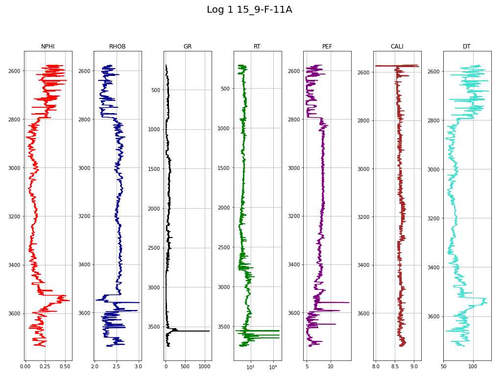
makeplot(log1,"Log 1 15_9-F-11A")
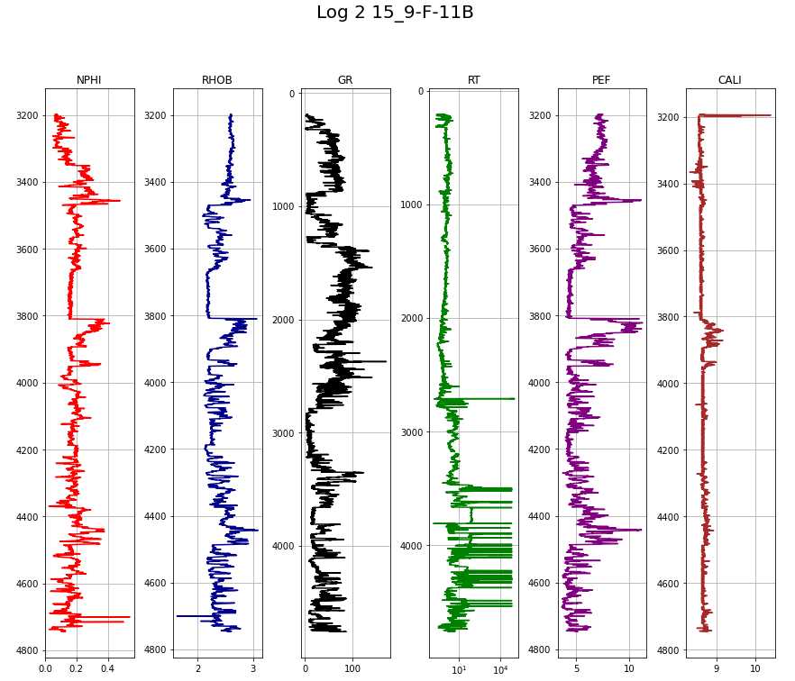
makeplot(log2, "Log 2 15_9-F-11B")
Data Preparation
- The train test split is easy, the data is already partitioned by wells:
- Train on logs 1, 3, and 4.
- Test (validation) on logs 2 and 5.
- There are many NAN values in the logs. The plots above only display the samples that are non-NaN and thus can be used to gauge where they need to be clipped. The NaN are primarily present on top and bottom of each log before readings start. The logs get clipped around the following depths:
- log1 2,600 - 3,720 m
- log2 3,200 - 4,740 m
- log3 2,620 - 3,640 m
- log4 3,100 - 3,400 m
- log5 3,100 - 4,050 m
- Furthermore, the logs contain many more featurs than we need. The correct will get selected for further use, the rest gets discarded.
# Lists of depths for clipping
lower = [2600, 3200, 2620, 3100, 3100]
upper = [3720, 4740, 3640, 3400, 4050]

# Lists of selected columns
train_cols = ['DEPTH', 'NPHI', 'RHOB', 'GR', 'RT', 'PEF', 'CALI', 'DT']
test_cols = ['DEPTH', 'NPHI', 'RHOB', 'GR', 'RT', 'PEF', 'CALI']

log_list_clipped = [0] * len(paths)

for i in range(len(log_list)):

  # Clip depths
  temp_df = log_list[i].loc[
      (log_list[i]['DEPTH'] >= lower[i]) &
      (log_list[i]['DEPTH'] <= upper[i])
  ]

  # Select train-log columns
  if i in [0,2,3]:
    log_list_clipped[i] = temp_df[train_cols]

  # Select test-log columns
  else:
    log_list_clipped[i] = temp_df[test_cols]

# Save logs from list into separate variables
log1, log2, log3, log4, log5 = log_list_clipped
# check for NaN
log1
| DEPTH | NPHI | RHOB | GR | RT | PEF | CALI | DT | |
|---|---|---|---|---|---|---|---|---|
| 24115 | 2600.0 | 0.371 | 2.356 | 82.748 | 1.323 | 7.126 | 8.648 | 104.605 |
| 24116 | 2600.1 | 0.341 | 2.338 | 79.399 | 1.196 | 6.654 | 8.578 | 103.827 |
| 24117 | 2600.2 | 0.308 | 2.315 | 74.248 | 1.171 | 6.105 | 8.578 | 102.740 |
| 24118 | 2600.3 | 0.283 | 2.291 | 68.542 | 1.142 | 5.613 | 8.547 | 100.943 |
| 24119 | 2600.4 | 0.272 | 2.269 | 60.314 | 1.107 | 5.281 | 8.523 | 98.473 |
| … | … | … | … | … | … | … | … | … |
| 35311 | 3719.6 | 0.236 | 2.617 | 70.191 | 1.627 | 7.438 | 8.703 | 84.800 |
| 35312 | 3719.7 | 0.238 | 2.595 | 75.393 | 1.513 | 7.258 | 8.750 | 85.013 |
| 35313 | 3719.8 | 0.236 | 2.571 | 82.648 | 1.420 | 7.076 | 8.766 | 85.054 |
| 35314 | 3719.9 | 0.217 | 2.544 | 89.157 | 1.349 | 6.956 | 8.781 | 84.928 |
| 35315 | 3720.0 | 0.226 | 2.520 | 90.898 | 1.301 | 6.920 | 8.781 | 84.784 |
Next Steps:
Concatenate the training logs into a training df and the test logs into a test df
Assign log/well names to each sample.
Move column location to the right.
# Concatenate dataframes
train = pd.concat([log1, log3, log4])
pred = pd.concat([log2, log5])

# Assign names
names = ['15_9-F-11A', '15_9-F-11B', '15_9-F-1A', '15_9-F-1B', '15_9-F-1C']

names_train = []
names_pred = []

for i in range(len(log_list_clipped)):
  if i in [0,2,3]:
    # Train data, assign names
    names_train.append(np.full(len(log_list_clipped[i]), names[i]))
  else:
    # Test data, assign names
    names_pred.append(np.full(len(log_list_clipped[i]), names[i]))

# Concatenate inside list
names_train = list(itertools.chain.from_iterable(names_train))
names_pred = list(itertools.chain.from_iterable(names_pred))

# Add well name to df
train['WELL'] = names_train
pred['WELL'] = names_pred

# Pop and add depth to end of df
depth_train, depth_pred = train.pop('DEPTH'), pred.pop('DEPTH')
train['DEPTH'], pred['DEPTH'] = depth_train, depth_pred

# Train dataframe with logs 1,3,4 vertically stacked
train
| NPHI | RHOB | GR | RT | PEF | CALI | DT | WELL | DEPTH | |
|---|---|---|---|---|---|---|---|---|---|
| 24115 | 0.3710 | 2.3560 | 82.7480 | 1.3230 | 7.1260 | 8.6480 | 104.6050 | 15_9-F-11A | 2600.0 |
| 24116 | 0.3410 | 2.3380 | 79.3990 | 1.1960 | 6.6540 | 8.5780 | 103.8270 | 15_9-F-11A | 2600.1 |
| 24117 | 0.3080 | 2.3150 | 74.2480 | 1.1710 | 6.1050 | 8.5780 | 102.7400 | 15_9-F-11A | 2600.2 |
| 24118 | 0.2830 | 2.2910 | 68.5420 | 1.1420 | 5.6130 | 8.5470 | 100.9430 | 15_9-F-11A | 2600.3 |
| 24119 | 0.2720 | 2.2690 | 60.3140 | 1.1070 | 5.2810 | 8.5230 | 98.4730 | 15_9-F-11A | 2600.4 |
| … | … | … | … | … | … | … | … | … | … |
| 32537 | 0.1861 | 2.4571 | 60.4392 | 1.2337 | 5.9894 | 8.7227 | 75.3947 | 15_9-F-1B | 3399.6 |
| 32538 | 0.1840 | 2.4596 | 61.8452 | 1.2452 | 6.0960 | 8.6976 | 75.3404 | 15_9-F-1B | 3399.7 |
| 32539 | 0.1798 | 2.4637 | 61.1386 | 1.2960 | 6.1628 | 8.6976 | 75.3298 | 15_9-F-1B | 3399.8 |
| 32540 | 0.1780 | 2.4714 | 59.3751 | 1.4060 | 6.1520 | 8.6976 | 75.3541 | 15_9-F-1B | 3399.9 |
| 32541 | 0.1760 | 2.4809 | 58.3742 | 1.4529 | 6.1061 | 8.6978 | 75.4476 | 15_9-F-1B | 3400.0 |
# Pred dataframe with logs 2, 5 verically stacked
pred
| NPHI | RHOB | GR | RT | PEF | CALI | WELL | DEPTH | |
|---|---|---|---|---|---|---|---|---|
| 30115 | 0.0750 | 2.6050 | 9.3480 | 8.3310 | 7.4510 | 8.5470 | 15_9-F-11B | 3200.0 |
| 30116 | 0.0770 | 2.6020 | 9.3620 | 8.2890 | 7.4640 | 8.5470 | 15_9-F-11B | 3200.1 |
| 30117 | 0.0780 | 2.5990 | 9.5450 | 8.2470 | 7.4050 | 8.5470 | 15_9-F-11B | 3200.2 |
| 30118 | 0.0790 | 2.5940 | 11.1530 | 8.2060 | 7.2920 | 8.5470 | 15_9-F-11B | 3200.3 |
| 30119 | 0.0780 | 2.5890 | 12.5920 | 8.1650 | 7.1670 | 8.5470 | 15_9-F-11B | 3200.4 |
| … | … | … | … | … | … | … | … | … |
| 39037 | 0.3107 | 2.4184 | 106.7613 | 2.6950 | 6.2332 | 8.5569 | 15_9-F-1C | 4049.6 |
| 39038 | 0.2997 | 2.4186 | 109.0336 | 2.6197 | 6.2539 | 8.5569 | 15_9-F-1C | 4049.7 |
| 39039 | 0.2930 | 2.4232 | 106.0935 | 2.5948 | 6.2883 | 8.5570 | 15_9-F-1C | 4049.8 |
| 39040 | 0.2892 | 2.4285 | 105.4931 | 2.6344 | 6.3400 | 8.6056 | 15_9-F-1C | 4049.9 |
| 39041 | 0.2956 | 2.4309 | 109.8965 | 2.6459 | 6.3998 | 8.5569 | 15_9-F-1C | 4050.0 |
Exploratory Data Analysis
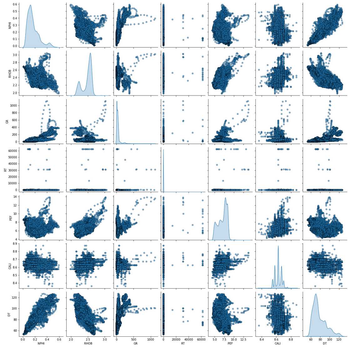
Pair-plot of the Train Data
train_features = ['NPHI', 'RHOB', 'GR', 'RT', 'PEF', 'CALI', 'DT']

sns.pairplot(train, vars=train_features, diag_kind='kde',
             plot_kws = {'alpha': 0.6, 's': 30, 'edgecolor': 'k'})
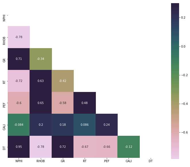
Spearman’s Correlation Heatmap
train_only_features = train[train_features]

# Generate a mask for the upper triangle
mask = np.zeros_like(train_only_features.corr(method = 'spearman') , dtype=np.bool)
mask[np.triu_indices_from(mask)] = True

# Custom colormap
cmap = sns.cubehelix_palette(n_colors=12, start=-2.25, rot=-1.3, as_cmap=True)

# Draw the heatmap with the mask and correct aspect ratio
plt.figure(figsize=(12,10))
sns.heatmap(train_only_features.corr(method = 'spearman'), annot=True,  mask=mask, cmap=cmap, vmax=.3, square=True)

plt.show()
Transformation of the Train Data
Normalize/transform the dataset:
- Log transform the RT log
- Use power transform with Yeo-Johnson method (except ‘WELL’ and ‘DEPTH’)
# Log transform the RT to logarithmic
train['RT'] = np.log10(train['RT'])

from sklearn.compose import ColumnTransformer
from sklearn.preprocessing import PowerTransformer

# Transformation / Normalizer object Yeo-Johnson method
scaler = PowerTransformer(method='yeo-johnson')

# ColumnTransformer (feature_target defines to which it is applied, leave Well and Depth untouched)
ct = ColumnTransformer([('transform', scaler, feature_target)], remainder='passthrough')

# Fit and transform
train_trans = ct.fit_transform(train)

# Convert to dataframe
train_trans = pd.DataFrame(train_trans, columns=colnames)
train_trans
| NPHI | RHOB | GR | RT | PEF | CALI | DT | WELL | DEPTH | |
|---|---|---|---|---|---|---|---|---|---|
| 0 | 1.702168 | -0.920748 | 1.130650 | -0.631876 | 0.031083 | 0.450019 | 1.588380 | 15_9-F-11A | 2600.0 |
| 1 | 1.573404 | -1.020621 | 1.092435 | -0.736154 | -0.373325 | -1.070848 | 1.562349 | 15_9-F-11A | 2600.1 |
| 2 | 1.407108 | -1.142493 | 1.030314 | -0.758080 | -0.819890 | -1.070848 | 1.525055 | 15_9-F-11A | 2600.2 |
| 3 | 1.260691 | -1.263078 | 0.956135 | -0.784153 | -1.197992 | -1.753641 | 1.460934 | 15_9-F-11A | 2600.3 |
| 4 | 1.189869 | -1.367969 | 0.837247 | -0.816586 | -1.441155 | -2.286221 | 1.367432 | 15_9-F-11A | 2600.4 |
| … | … | … | … | … | … | … | … | … | … |
| 24398 | 0.462363 | -0.279351 | 0.839177 | -0.704005 | -0.910619 | 2.041708 | 0.047941 | 15_9-F-1B | 3399.6 |
| 24399 | 0.439808 | -0.261621 | 0.860577 | -0.694407 | -0.826995 | 1.510434 | 0.043466 | 15_9-F-1B | 3399.7 |
| 24400 | 0.393869 | -0.232335 | 0.849885 | -0.653120 | -0.774093 | 1.510434 | 0.042591 | 15_9-F-1B | 3399.8 |
| 24401 | 0.373838 | -0.176628 | 0.822640 | -0.569367 | -0.782672 | 1.510434 | 0.044596 | 15_9-F-1B | 3399.9 |
| 24402 | 0.351335 | -0.106609 | 0.806807 | -0.535769 | -0.819021 | 1.514682 | 0.052292 | 15_9-F-1B | 3400.0 |
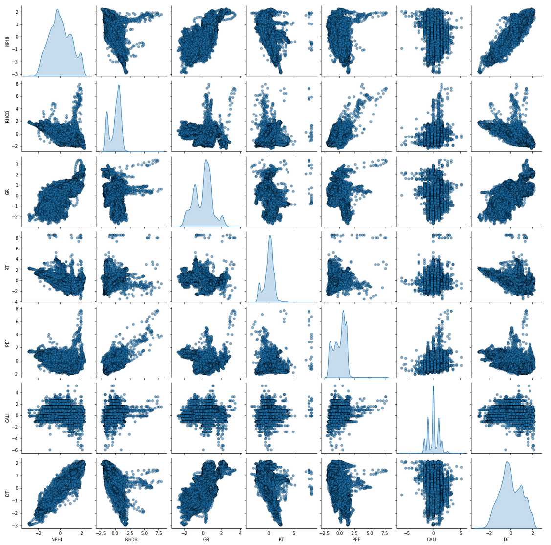
Pair-Plot (after transformation)
sns.pairplot(train_trans, vars=feature_target, diag_kind = 'kde',
             plot_kws = {'alpha': 0.6, 's': 30, 'edgecolor': 'k'})
Removing Outliers
Outliers can be removed easily with an API call. The issue is that there are multiple methods that may work with varying efficiency. Let’s run a few and select which one performs best.
from sklearn.ensemble import IsolationForest
from sklearn.covariance import EllipticEnvelope
from sklearn.neighbors import LocalOutlierFactor
from sklearn.svm import OneClassSVM

# Make a copy of train
train_fonly = train_trans.copy()

# Remove WELL, DEPTH
train_fonly = train_fonly.drop(['WELL', 'DEPTH'], axis=1)
train_fonly_names = train_fonly.columns

# Helper function for repeated plotting

def makeboxplot(my_title='enter title',my_data=None):
    _, ax1 = plt.subplots()
    ax1.set_title(my_title, size=15)
    ax1.boxplot(my_data)
    ax1.set_xticklabels(train_fonly_names)
    plt.show()

makeboxplot('Unprocessed',train_trans[train_fonly_names])
print('n samples unprocessed:', len(train_fonly))
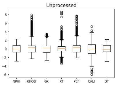
n samples unprocessed: 24,403
Method 1: Standard Deviation
train_stdev = train_fonly[np.abs(train_fonly - train_fonly.mean()) <= (3 * train_fonly.std())]

# Delete NaN
train_stdev = train_stdev.dropna()

makeboxplot('Method 1: Standard Deviation',train_stdev)
print('Remaining samples:', len(train_stdev))
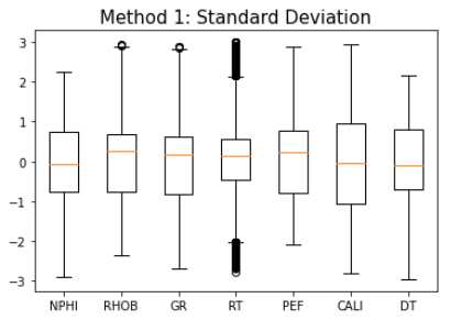
Remaining samples: 24,101
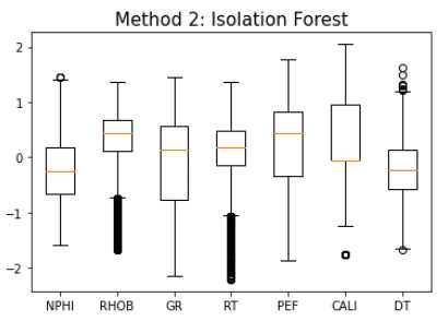
Method 2: Isolation Forest
iso = IsolationForest(contamination=0.5)
yhat = iso.fit_predict(train_fonly)
mask = yhat != -1
train_iso = train_fonly[mask]

makeboxplot('Method 2: Isolation Forest',train_iso)
print('Remaining Samples:', len(train_iso))
Remaining Samples: 12,202
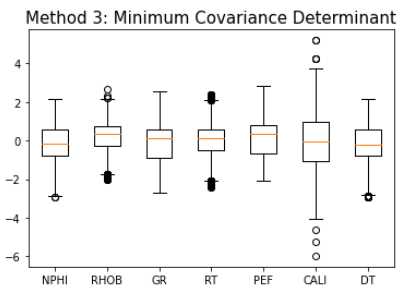
Method 3: Minimum Covariance Determinant
ee = EllipticEnvelope(contamination=0.1)
yhat = ee.fit_predict(train_fonly)
mask = yhat != -1
train_ee = train_fonly[mask]

makeboxplot('Method 3: Minimum Covariance Determinant',train_ee)
print('Remaining samples:', len(train_ee))
Remaining samples: 21,962
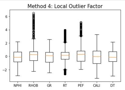
Method 4: Local Outlier Factor
lof = LocalOutlierFactor(contamination=0.3)
yhat = lof.fit_predict(train_fonly)
mask = yhat != -1
train_lof = train_fonly[mask]

makeboxplot('Method 4: Local Outlier Factor',train_lof)
print('Remaining samples:', len(train_lof))
Remaining samples: 17,082
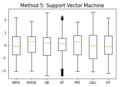
Method 5: Support Vector Machine
svm = OneClassSVM(nu=0.1)
yhat = svm.fit_predict(train_fonly)
mask = yhat != -1
train_svm = train_fonly[mask]

makeboxplot('Method 5: Support Vector Machine',train_svm)
print('Remaining samples:', len(train_svm))
Remaining samples: 21,964
One-class SVM performs best
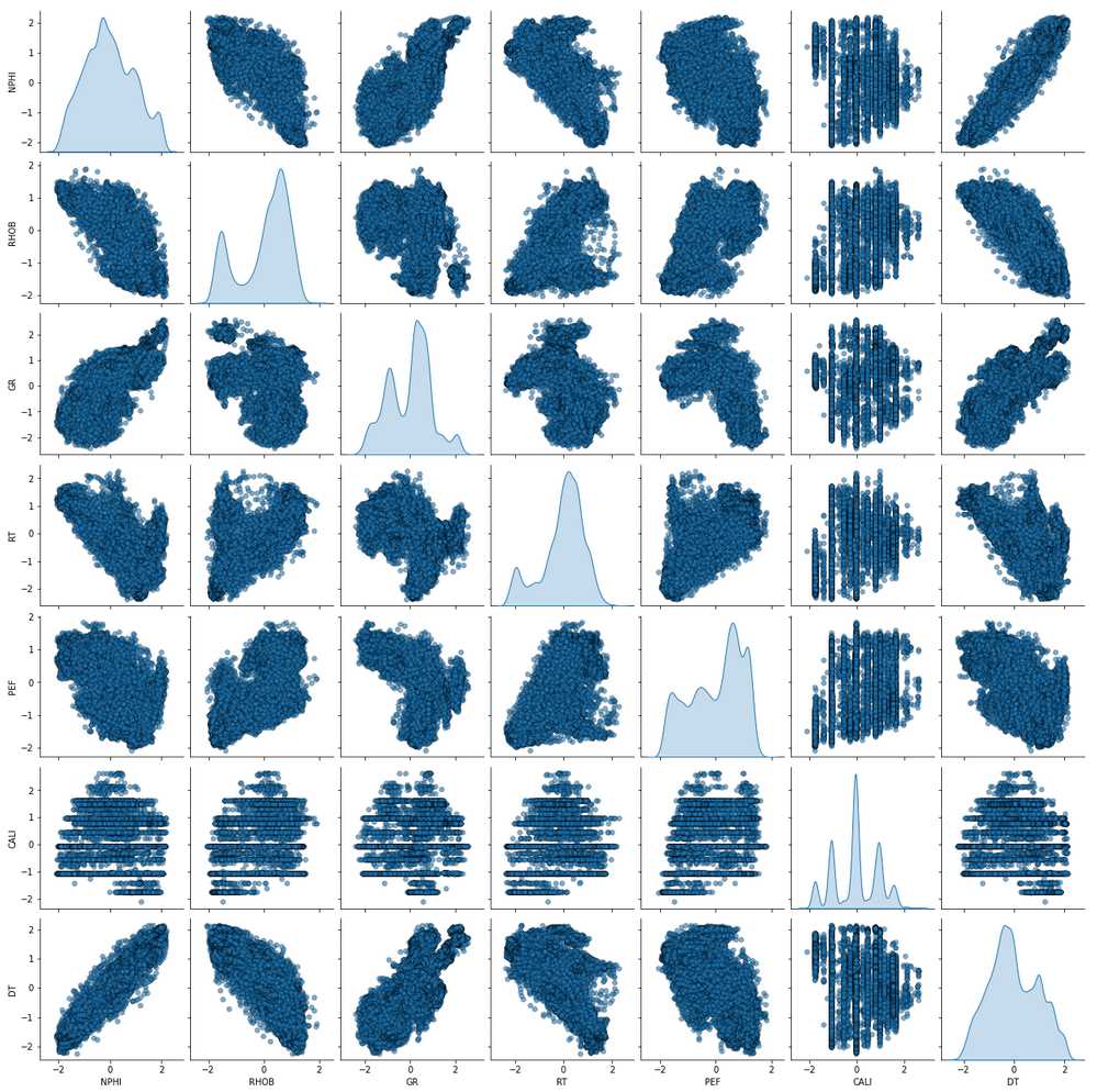
Make pair-plot of data after outliers removed.
sns.pairplot(train_svm, vars=feature_target,
             diag_kind='kde',
             plot_kws = {'alpha': 0.6, 's': 30, 'edgecolor': 'k'})
Train and Validate
Define the train data as the SVM outlier-removed-data.
# Select columns for features (X) and target (y)
X_train = train_svm[feature_names].values
y_train = train_svm[target_name].values

Define the validation data
train_trans_copy = train_trans.copy()

train_well_names = ['15_9-F-11A', '15_9-F-1A', '15_9-F-1B']

X_val = []
y_val = []

for i in range(len(train_well_names)):
  # Split the df by log name
  val = train_trans_copy.loc[train_trans_copy['WELL'] == train_well_names[i]]

  # Drop name column
  val = val.drop(['WELL'], axis=1)

  # Define X_val (feature) and y_val (target)
  X_val_, y_val_ = val[feature_names].values, val[target_name].values

  X_val.append(X_val_)
  y_val.append(y_val_)

# save into separate dfs
X_val1, X_val3, X_val4 = X_val
y_val1, y_val3, y_val4 = y_val
Fit to Test and Score on Val
from sklearn.metrics import mean_squared_error
from sklearn.ensemble import GradientBoostingRegressor

# Gradient Booster object
model = GradientBoostingRegressor()

# Fit the regressor to the training data
model.fit(X_train, y_train)

# Validation: Predict on well 1
y_pred1 = model.predict(X_val1)
print("R2 Log 1: {}".format(round(model.score(X_val1, y_val1),4)))
rmse = np.sqrt(mean_squared_error(y_val1, y_pred1))
print("RMSE Log 1: {}".format(round(rmse,4)))

# Validation: Predict on well 3
y_pred3 = model.predict(X_val3)
print("R2 Log 3: {}".format(round(model.score(X_val3, y_val3),4)))
rmse = np.sqrt(mean_squared_error(y_val3, y_pred3))
print("RMSE Log 3: {}".format(round(rmse,4)))

# Validation: Predict on well 4
y_pred4 = model.predict(X_val4)
print("R2 Log 4: {}".format(round(model.score(X_val4, y_val4),4)))
rmse = np.sqrt(mean_squared_error(y_val4, y_pred4))
print("RMSE Log 4: {}".format(round(rmse,4)))
R2 Log 1: 0.9526
RMSE Log 1: 0.2338
R2 Log 3: 0.9428
RMSE Log 3: 0.2211
R2 Log 4: 0.8958
RMSE Log 4: 0.2459
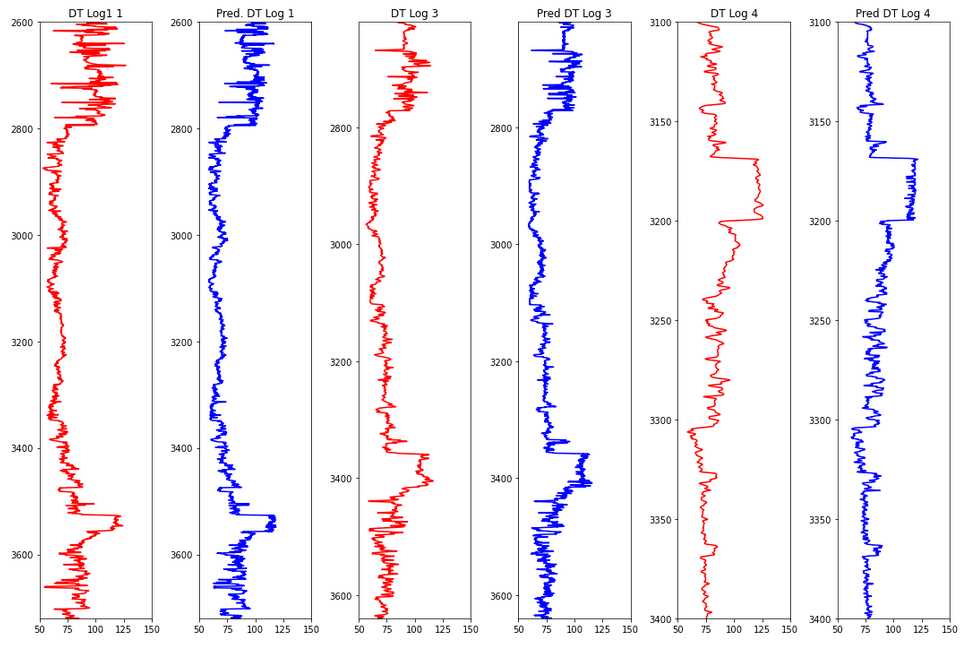
This R2 is relatively good with relatively little effort!
Inverse Transformation of Prediction
# Make the transformer fit to the target
y = train[target_name].values
scaler.fit(y.reshape(-1,1))

# Inverse transform  y_val, y_pred
y_val1, y_pred1 = scaler.inverse_transform(y_val1.reshape(-1,1)), scaler.inverse_transform(y_pred1.reshape(-1,1))
y_val3, y_pred3 = scaler.inverse_transform(y_val3.reshape(-1,1)), scaler.inverse_transform(y_pred3.reshape(-1,1))
y_val4, y_pred4 = scaler.inverse_transform(y_val4.reshape(-1,1)), scaler.inverse_transform(y_pred4.reshape(-1,1))
Plot a comparison between train and prediction of the DT feature.
x = [y_val1, y_pred1, y_val3, y_pred3, y_val4, y_pred4]
y = [log1['DEPTH'], log1['DEPTH'], log3['DEPTH'], log3['DEPTH'], log4['DEPTH'], log4['DEPTH']]

color = ['red', 'blue', 'red', 'blue', 'red', 'blue']
title = ['DT Log1 1', 'Pred. DT Log 1', 'DT Log 3', 'Pred DT Log 3',
         'DT Log 4', 'Pred DT Log 4']

fig, ax = plt.subplots(nrows=1, ncols=6, figsize=(15,10))

for i in range(len(x)):
  ax[i].plot(x[i], y[i], color=color[i])
  ax[i].set_xlim(50, 150)
  ax[i].set_ylim(np.max(y[i]), np.min(y[i]))
  ax[i].set_title(title[i])

plt.tight_layout()

plt.show()
Hyperparameter Tuning
This example below is GridSearchCV hyperparameter tuning on Scikit-Learn’s GradientBoostingRegressor, resulting in 31 models playing through all variations.
Different ways of searching hyperparameters are available with automated approaches of narrowing it down in a smarter way.
from sklearn.model_selection import train_test_split

# Define the X and y from the SVM normalized dataset
X = train_svm[feature_names].values
y = train_svm[target_name].values

# Train and test split
X_train, X_test, y_train, y_test = train_test_split(X, y, test_size=0.3, random_state=42)
The grid search will churn for several minutes and the best scoring parameter combination saved printed.
from sklearn.model_selection import GridSearchCV

model = GradientBoostingRegressor()

# Hyperparameter ranges

max_features = ['auto', 'sqrt']
min_samples_leaf = [1, 4]
min_samples_split = [2, 10]
max_depth = [10, 100]
n_estimators = [100, 1000]

param_grid = {'max_features': max_features,
              'min_samples_leaf': min_samples_leaf,
              'min_samples_split': min_samples_split,
              'max_depth': max_depth,
              'n_estimators': n_estimators}

# Train with grid
model_random = GridSearchCV(model, param_grid, cv=3)
model_random.fit(X_train, y_train)

# Print best model
model_random.best_params_
{‘max_depth’: 100,
‘max_features’: ‘sqrt’,
‘min_samples_leaf’: 4,
‘min_samples_split’: 10,
‘n_estimators’: 1000}
Predict Test Wells
Define the Test Data
# Define the test data
names_test = ['15_9-F-11B', '15_9-F-1C']

X_test = []
y_test = []
depths = []

for i in range(len(names_test)):
  # split the df with respect to its name
  test = pred.loc[pred['WELL'] == names_test[i]]

  # Drop well name column
  test = test.drop(['WELL'], axis=1)

  # Define X_test (feature)
  X_test_ = test[feature_names].values

  # Define depth
  depth_ = test['DEPTH'].values

  X_test.append(X_test_)
  depths.append(depth_)

# For each well 2 and 5
X_test2, X_test5 = X_test
depth2, depth5 = depths
Transform Test - Predict - Inverse Transform
# Transform X_test of log 2 and 5
X_test2 = scaler.fit_transform(X_test2)
X_test5 = scaler.fit_transform(X_test5)

# Predict to log 2 and 5 with tuned model
y_pred2 = model_random.predict(X_test2)
y_pred5 = model_random.predict(X_test5)

y = train[target_name].values
scaler.fit(y.reshape(-1,1))

# Inverse transform y_pred
y_pred2 = scaler.inverse_transform(y_pred2.reshape(-1,1))
y_pred5 = scaler.inverse_transform(y_pred5.reshape(-1,1))
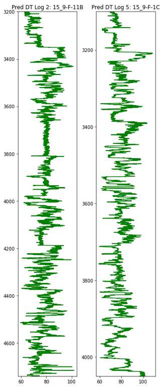
Plot the Predictions
plt.figure(figsize=(5,12))

plt.subplot(1,2,1)
plt.plot(y_pred2, depth2, color='green')
plt.ylim(max(depth2), min(depth2))
plt.title('Pred DT Log 2: 15_9-F-11B', size=12)

plt.subplot(1,2,2)
plt.plot(y_pred5, depth5, color='green')
plt.ylim(max(depth5), min(depth5))
plt.title('Pred DT Log 5: 15_9-F-1C', size=12)

plt.tight_layout()
plt.show()
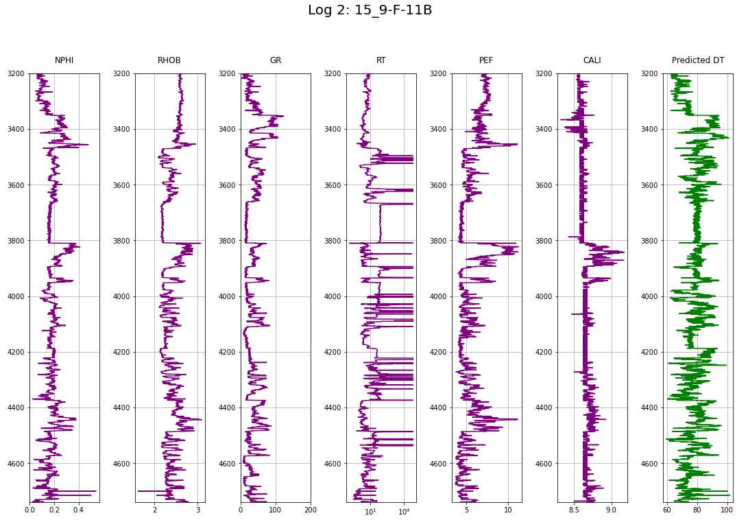
def makeplotpred(df,suptitle_str="pass a suptitle"):
  # Column selection from df
  col_names = ['NPHI', 'RHOB', 'GR', 'RT', 'PEF', 'CALI', 'DT']
  # Plotting titles
  title = ['NPHI', 'RHOB', 'GR', 'RT', 'PEF', 'CALI', 'Predicted DT']
  # plotting colors
  colors = ['purple', 'purple', 'purple', 'purple', 'purple', 'purple', 'green']

  # Create the subplots; ncols equals the number of logs
  fig, ax = plt.subplots(nrows=1, ncols=len(col_names), figsize=(15,10))
  fig.suptitle(suptitle_str, size=20, y=1.05)

  # Looping each log to display in the subplots
  for i in range(len(col_names)):
    if i == 3:
      # for resistivity, semilog plot
      ax[i].semilogx(df[col_names[i]], df['DEPTH'], color=colors[i])
    else:
      # for non-resistivity, normal plot
      ax[i].plot(df[col_names[i]], df['DEPTH'], color=colors[i])

    ax[i].set_ylim(max(df['DEPTH']), min(df['DEPTH']))
    ax[i].set_title(title[i], pad=15)
    ax[i].grid(True)

  ax[2].set_xlim(0, 200)
  plt.tight_layout(1)
  plt.show()
makeplotpred(log2,"Log 2: 15_9-F-11B")
makeplotpred(log5,"Log 5: 15_9-F-1C")
Remind me, how did that expression go? The following post consists of notes I had on my drive and I had been returning to over and over to remind me of some concepts and SQL syntax. Of course, the original tables and outputs are not available here, but the point is providing a lookup for structures and building blocks. The CASE statement can create a new column based on multiple conditions in a specified column. The structure always follows The following query creates multiple new columns with a summation aggregate function. For each country calculate the percentage of ties (home=away goals_). Use the Similar as in most languages, SQL can make use of Try/Catch (sometimes called exception/error blocks). It is also possible to have a nested TRY block inside the CATCH block, which lets you attempt a second query if the first failed. Use example: the nested (inner) TRY block could be used to write an error message into a table that the outer TRY failed. The following query writes a message to an ‘error’ table if the outer Try block fails. If that fails, too, then the error details of the inner try are queried. ‘RAISERROR’ lets you define a custom error and parameters. Syntax: While regular subqueries can be calculated on their own, correlated subqueries cannot need results from outer queries. Queries with multiple subqueries will get complicated quickly. Subqueries in Correlated subqueries reference one or more columns in the main query. They dend on information in the main query to run, and thus, cannot be executed on their own. Correlated subqueries are evaluated in SQL once per row of data retrieved - a process that takes a lot more computing power and time than a simple subquery. The following Now it’s getting complicated. Best design such queries from inner to outer. CTEs are declared and executed ahead of the main query and help organizing queries with complicated subqueries. They always precede the main query and go The The empty The following qerry with the Calculate a ranking and also order the query by rank. Note: Assigns the same number to rows with identical values and skips over the next numbers. E.g.: 1,2,3,3,5,6,6,8… The following query calculates the average goals per game and groups by league. The averages are ranked by league. Note: Assigns same number to rows with identical values but does NOT skip over the next numbers. E.g.: 1,2,3,3,4,5,5,6… Generate a column that counts the current The Keywords for sliding windows are The window is supposed to run sum and averages between the current row and the top of the table or bottom of the table. They both arrive at the same cumulative sum, but the way to get there is different. Difference The following query is calculating the Running Total (RT) and Running Aaverage (). The window uses ascending date ordering (smallest date number at top) -> the window goes from top (oldest date) of table to current row. The following query is calculating the RT and RA in descending date ordering (largest date number at top) -> the window goes from current row to bottom (oldest date). Moving average (MA). Calculate a column with the 3-year (2 preceding + current) average. The The following query determins (1) for each year’s Olympics which the gold medal country is and (2) which country is the reigning/last champion country. The These functions do not depend on the current row’s position. The following query fetches the gold-winner athlete and a second column with the first athlete. The order is alphabetically. Fetching the last value is more complicated, since it requires the definition of the Otherwise the last value of the window is the current row, and that’s now what we mean. Window functions can be applied to separate columns into processing sections. This way, it can be avoided that functions leak over from one section into another, e.g. when using The following query partitions the table by gender and avoids the Partition by multiple columns (gender and event). The following query subdivides the ordered medals into three pages. Perform aggregate function analysis on the pages/quantiles. The following query gets the average medals earned in each page. Pivoting with A regular query gets entered into the Original: Pivot by year: ROLLUP() vs CUBE() Use ROLLUP() for hierachical data such as data parts (year, quarter) and don’t wall all possible group-level aggregations. Use CUBE() for all possible group-level aggregations The following query counts medals by country and gender. At the gender group level there is a total row (male+female) using the Group totals by all possible groups with Useful for any function that produces nulls, such as Use in Use in Input Table: Output string: USA, RUS, AUS Merge strings with || CHARLOTTE HUNTER Another example: 1: CHARLOTTE HUNTER Merge strings with posgreSQL’s 1: CHARLOTTE HUNTER Police Academy If just the column string is passed to TRIM(), then all If no trim char string passed, is entered, then Syntax: ’#######[email protected]’, ‘[email protected]\(\)$’ [email protected], moc.goh@egdeh Police Academy, 14, 14 Remember, that SQL indexing starts at 1, not 0! [email protected], 6, 6 LEFT(), RIGHT(): Specify how many characters to be clipped starting from the ends. SUBSTRING()/SUBSTR(): Specify the start index and length. SUBSTRING(): Use functions to determine start/end index with FROM…FOR expression. hedge, hog.com Clip a column to 50 characters but do not clip a word in half. PostgreSQL native casting with two colons Standard SQL casting with A User-Defined Function is the equivalent of a Stored Proceedure. A function can bundle several SQL queries together into a package using 100 Postgre has extensions of the normal Additional features are stemming, fuzzy matching (spelling mistakes), and ranking. Calculate the Levenshtein Distance (number of edits required between two words). 3 Calculate Similarity (0-1) Drop duplicate rows based on specific columns, not the entire rows is duplicated. Use a Common Table Expression (CTE) with a window function ‘PARTITION BY’ that creates a row number per window. Any duplicates will have a row number >2. Then, evaluate the CTE and only keep row numbers = 1. This query selects a timestamp style column and performs arithmetic on it with the Convert integers to time intervals. The Two useful functions are Timestamp parts/fields to extract: Examples for the quarter of the year in a timestamp: 1 1 The following query extracts quarters and years from a timestamp column and sums the payment amount by by quarter and years. The following query extracts the rental duration (rental_days) in a time interval of 90 days starting from 2005-05-01. The 2009-01-01 00:00:00 2009-05-01 00:00:00 The following query truncates to a day and counts the number of entries (rentals) by day. Transactions move around values between owners. For example money between bank accounts. This means a transaction contains a subtraction and addition that both have to succeed. The concept of “Atomic transactions” rolls back a transaction if any of its parts raised an error. SQL has a specific ‘TRAN’ keyword that can be put in a ‘TRY’ block. If the ‘TRAN’ raised an error, the ‘CATCH’ block calls a ‘ROLLBACK TRAN’. With ‘SET XACT_ABORT ON;’ errors in a ‘TRAN’ block will always be rolled back. No ‘TRY’ block needed. Note: ‘THROW’ error still works with XACT_ABORT. It is not necessary to fetch the entire array of a column. We can select specific elements with square brackets. Indexing in PostgresSQL starts with 1, and not 0 as with many other languages. Search for text in ARRAY in specific position. Search for text in any ARRAY position with The SQL query is passed as a single string. The tripple quotation mark wrapping (“””) is useful to have multi-row strings in Python. The table name goes in quotation marks and the SQL server connection has to be passed after the query. Connection URI (Uniform Resource Identifier) for PostgreSQL: postgresql://[user[:password]@][host][:port][/database] Do some column transformations in Spark e.g., convert float to string and split on pattern into multiple columns. Loading into analytical PostgreSQL database Creating a table schema works with [column name] [data-type]. ARRAYS can be created with square brackets. Multiple square brackets are nested arrays. Inserting works with calling the column names if only specific columns are inserted into. Inserting multiple rows into all columns at once can be done without column names, but the order has to match the columns. ARRAYS are inserted with curly braces {} and array elements separated by commas. Which tables are in the system database? Which columns are in the ‘actor’ table and what are their details? Column descriptions are detailed: Available in the distribution ready to be installed. dblink, pg_stat_tatements, pg_trgm Currently installed and ready for use. plpgsql First install and then check if the installation succeeded. Summary from reading the Andreessen Horowitz blog The writeup below are some highlights I wrote for myself. If you find the writeup useful and want to know more, then you should absolutely read the article linked. This is my personal summary from reading The New Business of AI (and How It’s Different From Traditional Software), which was published on the Andreessen Horowitz blog a16z.com, a Silicon Valley venture capital (VC) investor. This VC supported the likes of Skype and Facebook when they were still little known and dozens of others whos digital services we are using in our daily lives. The article is excellently written, and part of the AI in 2020 series. This series is a distillation of dozens of interviews the authors lead with ML tams and thus marks a great resource for machine learning professionals who want deep insights into new AI developments, be it startups or mature companies. And last but not least it helps evaluating the next job opportunities. Most of all, the series is intended by Andreessen Horowitz to support AI companies, a sector in which they are investing heavily. Investors are betting today that AI companies will make a similar return as software companies. However, in many cases that AI companies have a different economic construction than software businesses: Lower gross margins -> heavy cloud infrastructure + human support Scaling problems due to edge cases. Weaker defensive moats -> commoditization of AI models and challenges with data network effects. Consistent pattern in the financial data of AI companies: gross margins 50-60% range, 60-80%+ for SaaS businesses. Early investors pushing AI companies for rapid growth over returns may obscure lower growth rates. AI is going to be a new type of business - after SaaS - and it is clearly different from Software. The differences have to be acknowledged and addressed. Software (including SaaS) can be produced once and sold many times. Benefits are: A) recurring revenue streams, B) high (60-80%+) gross margins, and C) super linear scaling with (rare) network effects, D) ownership of intellectual property (source code) builds defensive moats. Each new project requires dedicated headcount and can be sold exactly once: B) revenue is non-recurring, B) gross margins are lower (30-50%), C) and scaling is linear at best, D) Defensibility is challenging – often based on brand or incumbent account control – because any IP not owned by the customer is unlikely to have broad applicability. Appear to combine elements of both software and services. Most AI applications look + feel like normal software: interfacing with users, managing data, or integrating with other systems. However, at the center is a set of trained data models. Maintaining these models is more like a services business. That is: requiring significant, customer-specific work and input costs beyond typical support and success functions. AI is very demanding on cloud infrastructure: training, inference, and retraining due to data-drift, large file size input data and model transfer across cloud regions are more demanding than traditional software operations. Combined, 25% (or more) of revenue are spent on cloud resources. Manual processing can be cheaper in a company’s early start-up phase. Model complexity is growing at fast rate. 10x data is needed for 2x model precision. CPU/GPUs cannot be accelerated and made cheaper fast enough. Distributed computing solves speed issues, but not costs. Training most of today’s state-of-the-art AI models involves the manual cleaning and labeling of large datasets. This process is laborious, and expensive. For many tasks, especially those requiring greater cognitive reasoning, humans are often plugged into AI systems in real time. The need for human intervention will likely decline as the performance of AI models improves. It’s unlikely that humans will be removed entirely. How much will margins increase with AI fully automated? Reducing human intervention (and their costs) will likely increase cloud costs. New customers increases the work for the ML team when the models have to be adjusted for these new customers -> drawing resources away from new sales. The problem is edge cases. Many AI apps have open-ended interfaces and operate on noisy, unstructured data (e.g., images, NLP). Handling edge cases means endless possible input values. Each new customer deployment is likely to infer on completely new data. AI companies spend time re-training the model for each new customer to eliminate edge cases prior to deployment until accuracy reaches acceptable levels. Startups spend more time + resources for deployment than expected. Identifying challenges in advance can be difficult since traditional prototyping tools (mockups, prototypes, beta tests) do not cover edge cases. Some of the best defensive moats are network effects, high switching costs, and economies of scale. Additionally, branding comes from first to market and near-exclusivity. For AI players, differentiation is harder: New model architectures are developed mostly in open, academic settings. Reference implementations (pre-trained models) are available from open-source libraries, and hyperparameters can be optimized automatically. While data is at the heart of AI, it is often owned by customers, in the public domain, or over time becomes a commodity. Moats for AI companies appear to be shallower than for software and shallower than expected. Reduce model complexity: If possible, share a single model (or set of models) among all customers. It is easier to maintain, faster to roll out, and supports a simpler, more efficient engineering organization. Result: minimize cloud costs. Choose problem domains carefully and narrowly: The minimum viable task for AI models is narrower than expected. Choose problems that are hard for humans but easy for AI. That is high scale, low complexity tasks. Plan for high variable costs: build a business model and Go-To-Market strategy with lower gross margins in mind. Understand the distribution of the model data. Model maintenance and human failover are first-order problems. Measure real variable cost (no hiding in R&D). Make conservative assumptions in financial models (esp. fundraise). Scale and (outside) tech advances may not solve the problem. Embrace services: Building hybrid businesses (software/AI plus service) is harder than pure software, but this approach can provide deep insight into customer needs and yield fast-growing, market-defining companies. Plan for change in the tech stack: AI is still new. Standardized tools are just now being built: tools to automate model training, make inference more efficient, standardize developer workflows. Tightly coupling an application to the current state may lead to an architectural disadvantage in the future. Build defensible: It is unclear whether an AI model or the underlying data is a long-term moat. Good products and proprietary data almost always build good businesses. AI may vitalize old markets. Effective cloud strategies are key. Most AI systems are not like software and such the business works differently. AI businesses scale not as easily, and it is harder to build defensibility. Taken together, that makes AI feel more like a service business. These are unfamiliar patterns, which indicate that AI companies are truly something new, including massive opportunities. Summary from reading the Andreessen Horowitz blog The writeup below are some highlights I wrote for myself. If you find the writeup useful and want to know more, then you should absolutely read the article linked. This is my personal summary from reading Taming the Tail: Adventures in Improving AI Economics, which was published on the Andreessen Horowitz blog a16z.com, a Silicon Valley venture capital (VC) investor. This VC supported the likes of Skype and Facebook when they were still little known and dozens of others whose digital services we are using in our daily lives. The article is excellently written, and part of the AI in 2020 series. This series is a distillation of dozens of interviews the authors lead with ML tams and thus marks a great resource for machine learning professionals who want deep insights into new AI developments, be it startups or mature companies. And last but not least it helps evaluating the next job opportunities. Most of all, the series is intended by Andreessen Horowitz to support AI companies, a sector in which they are investing heavily. AI companies is different from traditional software companies. Often they have lower margins, are harder to scale, and don’t always have strong defensive moats. (…in the presence of long-tailed data distributions) Traditional software is a task of engineering. The specifications of a product are defined and then slowly added to the software - one line of code at a time. AI developers build statistical models, measure them, build a new one, measure, and so on. Until a satisfactory quality threshold was crossed, the AI modeler has to go through this experimentation loop. The article quotes an AI CTO that the process is “closer to molecule discovery in pharma” than engineering. Another issue is that the code written by the AI developer only indirectly influences the output, which adds an additional layer of complexity. It mainly governs how the dataset is processed, but the quality of the outcome is unsure. Many ML natural datasets have a long-tailed (skewed) frequency distribution. The long tail makes up ~70% of the total amount of samples. This makes it when picking randomly much more likely to receive a sample from the tail. Head and Middle, where the most common samples are, receive only 30% of picks. However, the low-frequency samples from the tail are harder to train with supervised learning, while value is relatively low. These long-tail samples are often also called “edge cases” and are much harder to get right. Improving models on the long tail costs a lot of compute resources and thus creates more (cloud) costs than traditional software would cause (3-5x higher). Data has a cost to collect, process, and maintain. That means the larger the long-tailed dataset becomes, the harder it becomes to work with it and more costly, too. The projects actually show “DISeconomies of scale”. While more data to improve a model is often available, the long-taildness also means a diminishing return. AI developers may need 10x more data to achieve a 2x subjective improvement. While computing power becomes cheaper and more available (Moore’s Law), this does not occur with model performance at the moment. Economics of AI are a function of the problem (dataset modeling/characterizing causes computing costs), not part of the technology used (computing efficiency gains). Hence, the approach of the long-tail frequency distribution has to be optimized. First of all, it has to be determined if a long-tailed frequency dataset is there at all. If not, then no ML or DL should be used. Linear or Polynomial Regression will be much more efficient. Logistic Regression and Random Forests are popular because they are A) interpretable, B) scalable, C) computationally efficient. DL may have its use cases in NLP (text generation and understanding), sentiment analysis but accuracy improvement has to be tightly balanced with training and maintenance costs. ML is not always the best solution to everything, which should be very closely evaluated. Heuristic and if/then approaches may be much easier to implement. Serving a single (global) model if there is large customer-segment/region overlap is much cheaper than building multiple models. -> “One size fits all” Tactics to build around the long tail: Componentizing: Train different simpler models to do different jobs concurrently. Example: Couldflare using 7 models to detect 6-7 different bot types attacking websites. Each model is global, and relatively easy to maintain. It is common to observe local problem (data) variation with customers, which do have to be addressed. Effort in modeling is based on the degree of local variation (countries, specific large customers….). Example: streaming services generating playlist models for each country. How to bring the benefits of global models to local problems? Operational best practices to improve AI economics: AI is still in its early years and has not yet crossed the peak of the hype cycle. More efficiency is needed. Structures similar to software development will likely appear Reasons that make ML experts look at your code twice. Strange and hard-to-read code is a common reason to elicit refactoring (rewriting). Think of unstructured Spaghetti Code™ without a lot of documentation – or the opposite – too much documentation that you can’t see the forest for the trees anymore. These kind of code issues are called “code smell”. A term that has been widely adopted after 1999 when the book “Refactoring: Improving the Design of Existing Code” by Martin Fowler was published. Its essence, refactoring is applying a series of small behavior-preserving transformations with the cumulative effect of “reducing the risk of introducing errors”. Some smells are easy to spot, some subtler and more insidious than others. While these problems and signs may not be detrimental by themselves, they warrant a closer look. You may have seen some of them before: Have a look at the full list of code smells and their description on Wikipedia and what Anupam Chugh discusses in his TowardsDataScience post “5 Python Code Smells You Should Be Wary Of”. At the time of writing this, Google Search users from Washington state were the most interested in code smells or at least ranking very highly. Check now on Google Trends. Is their code the smelliest of them all? Interest likely correlates with the amount of coders in a state and inevitably there is problematic code among. Photo by @claybanks on Unsplash Almost all Machine Learning entails someone writing code. This means the known problems or smells may be emanating from the codebase - regardless if we have written it or someone else put it into a black box for us to call. Machine Learning models are traditional functions but are mathematically adhering to different paradigms: a function that relates sample value X to some target value y. While all the functions of a comprehensive ML/DL library such as PyTorch, TensorFlow, and Scikit-learn are hopefully optimized and free of code smells under the hood, a project involves more than just a single algorithm that’s invoked in a single function. The workflow of invoking the library’s functions bespoke to our project’s needs is a “metamodel” with design complexities of its own. So what are the “ML smells” that might alert us to deeper problems in our prediction tools? Dr. Matt Hall recently asked the following question on Twitter and in the geological machine learning community Software Underground he co-founded: 🐽 ML smell is probably not a thing, but maybe it should be. What are the superficial signs of potentially deeper problems in a #machinelearning project?— Matt Hall (@kwinkunks) October 7, 2020 Matt crowdsourced some excellent responses: Black-box services such as AutoML. Counterintuitive model weights -> known effects have low feature importance. (Reece Hopkins, Anchorage) Unreproducible, non-deterministic code -> not setting random seeds. (Reece Hopkins, Anchorage) No train–val–test split description/justification. Leakage between training and blind data is easy to introduce with random splits in spatially correlated data. (Justin Gosses, Houston) No evaluation metric discussion -> how it was selected or designed (Dan Buscombe, Flagstaff) No ground truth discussion and how the target labels relate to it. (Justin Gosses, Houston) Excessive hyperparameter precision -> might suggest over-tuning. (Chris Dinneen, Perth) Precision–recall trade-off not considered -> especially in a binary classification task. (Dan Buscombe, FLagstaff) Strong class imbalance and no explicit mention of how it was handled. (Dan Buscombe, Flagstaff) Skewed feature importance on one or two features might suggest feature leakage. (John Ramey, Austin) Making excuses -> “we need more data”, “the labels are bad”, etc. (Hallgrim Ludvigsen, Stavanger) Time spend cleaning data too short -> Less than 80-90% of the effort spent on preparing the data. (Michael Pyrcz, Austin) Very high accuracy, e.g., 0.99 for a complex model on a novel task. (Ari Hartikainen, Helsinki and Lukas Mosser, Athens). In most real-world scenarios accuracy near 0.7 is excellent, and anything >0.8 indicates something unusual going on. That’s a long list, but there are most likely more. Most likely we have our own biases and tendencies to produce some smell because we were not aware, did not know any better, or had no other choice. This is where peer review provides a second (or third, or fourth…) pair of eyes is critical and all smells get cleaned up. What do you think? How perfect is your ML code and what kind of surface phenomena have you seen that may indicate deeper-rooted problems in ML projects? Maybe it is time for someone to officially coin a new term called “ML Smell”….. Thank-you to Matt Hall whose question inspired me to write this up! Don’t build from scratch! You want: This is going to easy, because this is a LaTeX template that has your needs covered. You are going to build the documents from source code by yourself. The template code is an evolution of the “Friggeri CV”, which was later substantially enriched in features by Jesper Dramsch in his repo “latex-cv-boosted”. If this sounds compelling, then head over to the GitHub repository to learn more. Not even that…. good. I love watching science-fiction films. In fact, as Student Union President during my Master’s I used to organize geology-related films about which whe had recently rearned in lectures. At least geology-related science-fiction films are usually so bad that they are good again: The Core, 2012, San Andreas, Dante’s Peak etc. Just for reference, in The Core the main characters used a giant drill through magma in the earth to jump-start the metal core’s rotation…. cough. Whenever I watch a sci-fi movie from a field I am less familiar with, I find it exciting to learn if the plot was at least marginally in accordance with the laws of nature. Honestly, there exits the full breadth of science-accuracy delivered by Hollywood from almost-documentary to completely bogus fluff. In my opinion, the Goldilocks situation is met if they achieve to combine excitement and awe with a reasonable adherence to laws of nature, e.g. “Jurassic Park”. For the past New Years days I made it an occasion to re-watch “Interstellar” – a gem in the astrophysics realm I had already seen in the theater when it was released. Most of the plot seemed relatively plausible to me. But I am not an astrophysicist, and what do I know about the details of General Relativity? So let’s find out what the the professor of astrophysics at North Carolina State University, Dr. Katie Mack, has to say in her review for the World Science Festival. Cinema Peer Review: Astrophysicist Katie Mack Reviews ‘Interstellar’ Well, returning from that read, I’m glad that Matthew McConaughey is still with us and did not have to be spaghettified. Dr. Mack brought up numerous pain points that I did not realize they were there. Ach, you were the chosen one, Interstellar. Scientific American: In “2012” neutrinos melt Earth’s core, and other disasters American Geophysical Union: Cinema Peer Review: Astrophysicist Katie Mack Reviews “Interstellar” GeoTimes: Watching The Core: A movie review Arizona Geological Survey: Review: San Andreas – The Movie What I read in 2020. Whenever I am looking for a new book to read, I really enjoy looking at lists of books other people read. Since I started reading more again this year (covid19…), I thought it would be a good idea to write down some thoughts on the individual books. I ended up picking up a new book almost every month. In the following, I describe the more interesting ones of them. Reinforcement learning is a subarea of Machine Learning with some essential differences to (un)supervised learning. The fundamental idea is that we want to train an agent that learns how to perform tasks in a dynamic environment. In contrast to supervised learning, the feedback given to the agent is delayed and does not tell it what the best action would have been. Because reinforcement learning is a bit of a niche area in Machine Learning, I never really got into it when I was new to the field. Still, the fundamental idea sounded incredibly interesting to me, so in the holidays after the winter semester I decided to work through this book. This was just in time to read the reworked second edition. The book was written by Sutton and Barto who are renowned experts in the field and came up with many of the most important ideas themselves. While the book does contain a large amount of math, it is still very accessible because everything is explained up from the ground up. Mentally processing the book was a lot of fun and I got a lot of inspiration for the future. Reinforcement learning is the key element in the AWS Deep Racer and I still marvel at the way it builds up the entire framework step by step. A Dance with Dragons is the fifth book from the A Song of Ice and Fire series that Game of Thrones is based on. After I read the first four book in 2015–2017, I was planning to read the other last book this year just so that I would be done when the sixth book was going to come out. Unfortunately, that book got delayed further and further and is not even out by now. All in all, I really enjoyed the book and its excruiciating details that greatly tops the TV series. Remembering all the >100 characters per book is not that easy, as Martin loves to explain backstory that does not really pertain to the plot. The writing style is neihter too dramatic nor withdrawn and I enjoy how each chapter is told from the point of view of a different character. However, sometimes story lines in some threads is not touched in a long time and comes up perhaps once in a book. Then it sometimes is better to get a reminder what was going in that corner of the world a couple hundred of pages ago. The Master Algorithm is a pop-scientific book about machine learning. It gives a nice overview of fundamental concepts and talks about the history of the field. The book is written for a general audience and does not assume prior knowledge. Domingos uses a lot of analogies, some of which were great, while some did not hit the nail on the head, I think. However, it is evident that he put in a lot of effort into trying to explain machine learning to people that are not from the field. The fundamental idea behind the book is that there are five different schools of thought in machine learning. These are the evolutionist, Bayesian, analogist, symbolist, and the currently dominating connectionist approach. Domingos argues that if we want to create a master algorithm that matches the learning power of our brain, ideas from all these tribes ought to be combined. The first part of the book introduces the five tribes and their main ideas. This was the strongest part of the book and I will probably go through this again at some point. The second part attempts to describe how they could be combined. This feels a bit forced and felt fairly abstract, since it is not entirely clarified how this should work. The book gives a good overview of subcultures and interests and tries to explain why some people feel drawn to them and coding in general. Thompson introduces the reader to coder culture and highlights a few case-study personalities he interviewed. He starts out with early history, such as computation at university servers, and later programming at home. Large part of the book is analyses of students in Computer Science programs and societal groups dominating the profession. In general, the book gives a good overview of subcultures and interests and tries to explain why some people feel drawn to coding in general. But it is never too technical to scare off people not familiar with the subject matter, I felt. The Sense of Style is a style guide that tries to explain how to write more elegantly and effectively. Now, there is no lack for how to write effectively, technical, scientifc, fast etc. However, Pinker’s work, Prof at Harvard U. Psychology Departmet, was smart enough to keep me reading – finding it even enjoyabl Partly, this is definitely because it is written by a highly eloquent author, which helps building your own style. The book addresses not only stylistic choices but also dives into more psychological aspects. One of these points that I really internalized is what the author calls the curse of knowledge. By having a deep understanding of a topic, it becomes incredibly hard to explain it in a good way to people without much prior knowledge. This is due to the fact that we forget the difficulties we had when first learning about the topic ourselves. Now it all seems so simple and it’s easy to fall into the trap of thinking that certain parts are also obvious to other people. Machine Learning’s ‘Hello World V2’ Dataset with Clothing. In 2017, Zalando Research published a dataset, which is very similar to the well known “Hello World” of Computer Vision: the MNIST database of handwritten digits. The dataset is designed for machine learning classification tasks and contains in total 60,000 training and 10,000 test images (gray scale) with each 28x28 pixel. Each training and test case is associated with one of ten labels (0–9). Up till here Zalando’s dataset is basically the same as the original handwritten digits data. However, instead of having images of the digits 0–9, Zalando’s data contains (not unsurprisingly) images with 10 different fashion products. Consequently, the dataset is called Fashion-MNIST dataset, which can be downloaded from GitHub or Kaggle. A few examples are shown in the following image, where each row contains one fashion item. The 10 different class labels are: According to the authors, the Fashion-MNIST data is intended to be a direct drop-in replacement for the old MNIST handwritten digits data, since there were several issues with the handwritten digits. For example, it was possible to correctly distinguish between several digits, by simply looking at a few pixels. Even with linear classifiers it was possible to achieve high classification accuracy. The Fashion-MNIST data promises to be more diverse so that machine learning (ML) algorithms have to learn more advanced features in order to be able to separate the individual classes reliably. Since the structure of the files in the Fashion-MNIST data is the same as for the old MNIST data, it is easy to load the new data with the older code. Using Additionally, I added a function (quick & dirty code) to visualize a sample of training images. The function basically samples the training data and shows random images in a squared grid. If desired, the images are arranged in a way that each row contains only samples from one class: For example, with Overall, the Fashion-MNIST dataset is an interesting test-bed for beginners in machine learning to apply different already existing algorithms. More advanced data scientists could use this data for a fast first evaluation of new approaches. However, this dataset is too simple to deliver reliable/comparable performance measures for new machine learning algorithms. Although I did not test it yet myself, I expect that simple convolutional neural networks would achieve an accuracy of around 90% on the Fashion-MNIST test data. More advanced neural networks can probably achieve an accuracy higher than 95%. For comparison, according to Zalando Research, the human performance is about 84%. Can you recognize some fashion items in the following matrix (although they are that tiny)? Our poor ML algorithms sometimes have to do this millions of times per day. Basic prinicples you need to know. In the previous articles about Machine Learning (ML) I touched advanced topics such as Computer Vision, Tensorflow Cats Vs Dogs I, Chat Bots, and many more. However, I never got into the nitty gritty details how Data Scientists and Machine Learning Enginneers deal with the model training and the maths behind the curtain. Let’s get to it now: Often it is impossible or impractical to compute certain values exactly to the last digit. This might be because it would take too long computationally or because we do not have not enough information. Instead, these values can be Estimation theory is useful to understand different versions of gradient descent. Typically, the gradient is only estimated using methods like (1) mini-batch or (2) stochastic gradient descent. Here, estimation theory can be used to explain the ideas behind these techniques. An estimator is a function (provided by your ML library) that estimates a value based on other observations. This process can involve randomness. For example, because the function itself is random or because there is random noise in the observations it uses. One measure for the quality of an estimator \(\tilde{X}\) (sometimes called \(\hat{X}\)) is its bias or how far off its estimate is on average from the true value \(X\): \[\begin{aligned} \mathrm{bias} ( \tilde{X} ) = \mathrm{E} \lbrack \tilde{X} \rbrack − X \end{aligned}\] where the expected value is over the randomness involved in \(\tilde{X}\). If the bias of an estimator is \(0\), it is called an unbiased estimator. This is generally a desirable property to have because it means that the estimator is correct on average. If one samples for long enough from the estimator, the average converges to the true value \(X\). This is due to the law of large numbers - but in reality we rarely have this luxury, unless we can horde immense amounts of data. Theorem: If \(k\) estimators all produce unbiased estimates \(\tilde{X}_1, \dots, \tilde{X}_k\) of \(X\), then any weighted average of them is also an unbiased estimator. The full estimate is given by \[\begin{aligned} \tilde{X} = w_1 * \tilde{X} _1 + \dots + w_k * \tilde{X} _k \end{aligned}\] where the sum of weights \(\textstyle\sum_{i=1}^k w_i = 1\) needs to be normalized. Proof: The unbiasedness is due to the linearity of expectation: \[\begin{aligned} \mathrm{E} \lbrack \tilde{X} \rbrack &= \mathrm{E} \lbrack w_1 * \tilde{X} _1 + \dots + w_k * \tilde{X} _k \rbrack \\[2em] &= w_1 * \mathrm{E} \lbrack \tilde{X} \rbrack + \dots + w_k * \mathrm{E} \lbrack \tilde{X} _k \rbrack \\[2em] &= w_1 * X + \dots + w_k * X \\[2em] &= X \\[2em] \end{aligned}\] This theorem about unbiased estimators is going to prove to be useful later. However, even if we have an unbiased estimator, its individual estimates can still be far off from the true value. To quantify how consistently an estimator is close to the true value, another statistic is required. Commonly, the variance of the estimator is considered here: \[\begin{aligned} \mathrm{Var} \lbrack \tilde{X} \rbrack = \mathrm{E} \lbrack ( \tilde{X} _k - X ) ^2 \rbrack \end{aligned}\] It is defined as the mean squared distance between the estimate and the value to be estimated. Many different things can be analyzed using estimators. For example, statistical and ML models can be seen as estimators. They use observations (samples, data…) to make predictions. These predictions are generally not perfect because randomness is involved and only a limited amount of information is available. Thus, it makes sense to analyze statistical models in terms of bias and variance. A central problem when building models is balancing underfitting and overfitting. If the training data is just memorized, the model does not generalize well to new data. This is a case of overfitting. The opposite issue, only barely matching the pattern in the training data, is called underfitting. This problem is also known as the bias-variance tradeoff: If the model has a high bias, its predictions are off, which corresponds to underfitting. If overfitting occurred, i.e., the data is learned too well, the estimates have a high variance. By resampling the data that the model was built on, totally different estimates are generated. This is because the model is now based on different random noise. Generally, it is not possible to perfectly optimize both, bias and variance, so they need to be balanced here. In other words, we accept a certain bias of the model to keep its variance low. A good tradeoff between the two needs to be achieved. In supervised machine learning, we compare our model’s predictions to the true labels. This is done using a loss function. If a set of data points \(x_1, \dots , x_n\) and labels \(y_1, \dots , y_n\) is given, then the full loss is defined by \[\begin{aligned} L = \frac{1}{n} \sum_{i=1}^n \mathrm{loss} (f(x_i),y_i) \end{aligned}\] where \(\mathrm{loss}\) is a function that compares a prediction \(p\) to the correct answer \(y\). One choice for the loss function might be the quadratic error (or Mean Absolute Error, Mean Squared Error, Median Absolute Error… etc.): \[\begin{aligned} \mathrm{loss} (p,y) = (p-y)^2 \end{aligned}\] Gradient descent optimizes the parameters used in \(f\) by computing the gradient of the loss with respect to these parameters. This gradient is then used to continually improve the parameters step by step during the descent. To compute the gradient \(ΔL\) of the loss, we can make use of the linearity of the gradient operator: \[\begin{aligned} ΔL &= Δ\frac{1}{n} \sum_{i=1}^n \mathrm{loss}(f(x_i),y_i) \\[2em] &= \frac{1}{n} \sum_{i=1}^n Δ \mathrm{loss}(f(x_i),y_i) \end{aligned}\] The method that uses the gradient given above is sometimes referred to as full-batch gradient descent because it fully uses the available training data in each iteration. Sometimes it also only called “Batch Gradient Descent” but that can be imprecise and confusing. In many cases, the full set of samples \(n\) is a very large value and computing the full update \(ΔL\) is expensive. Since computing the gradient is by far the most expensive part of gradient descent, it makes sense to try to make this more efficient. Computing the gradient as shown above is especially inefficient if there is duplicated training data. If the training set consists of 10 copies of a different dataset, then the evaluation of the formula above is unnecessarily expensive. Every required calculation is repeated 10 times. While this is an extreme example, it does happen in practice that much of the training data is similar. To save time, it often makes sense to only use a part of the data to estimate the gradient. In stochastic gradient descent (SGD), one single data point \(x\) and label \(y\) are sampled uniformly from the training set. This makes it the opposite extreme of Full-Batch Gradient Descent. The true gradient \(ΔL\) is then estimated using only this one data point and label: \[\begin{aligned} Δ\tilde{L} = Δ \mathrm{loss} (f(x),y) \end{aligned}\] It is easy to see that \(Δ\tilde{L}\) is an unbiased estimator of \(ΔL\): \[\begin{aligned} \mathrm{E} \lbrack Δ \tilde{L} \rbrack &= \sum_{i=1}^n Δ \mathrm{loss} (f(x_i),y_i) \\[2em] &= \frac{1}{n} Δ \sum_{i=1}^n \mathrm{loss} (f(x_i),y_i) \\[2em] &= ΔL \end{aligned}\] The computations for SGD can be performed very quickly but still give us an unbiased estimate of the true gradient. This property is the reason why optima can be found using this algorithm. While individual estimates are off, the randomness averages out over iterations and the parameters still move in a sensible direction overall. Since iterations are much cheaper, many more of them can be performed and this is a major improvement to computing the full gradient. These individual SGD estimates can have a large variance however, leading to noisy and jumpy gradients that show as zig-zaggy training histories. A further improvement over this method is mini-batch gradient descent. Instead of just taking one sample, we sample a small batch of \(k\) samples \(1 < k \ll n\), which makes it a compromise between Full-Batch Gradient Descent and Stochastic Gradient Descent. The estimated gradient is an average of all \(k\) single estimates. Each of these individual estimators is unbiased since SGD itself is unbiased. As shown in the theorem earlier, a weighted combination of them still remains an unbiased estimator. Thus, mini-batch gradient descent is also an unbiased way of computing gradient estimates. Mini-batch gradient descent does have much less variance, however, because more data is used to compute the estimate. This makes the optimization process less noisy and smoother compared to using SGD. Most gradient computations can be formulated using linear algebra operations. These calculations can be vectorized (parallelized very well on grphics cards that with CUDA (Don’t wait for hours). So with appropriate add-in boards for your computer there is no significant performance penalty for using Mini-Batch Gradient Descent to compute the model. Thus, Mini-Batch Gradient Descent is the preferred method that leads to a more stable optimization process. If you liked this mathematical representation of the formulas in this article and would like to adopt it, check out https://katex.org/, a LaTeX implementation for the web. It is implemented via 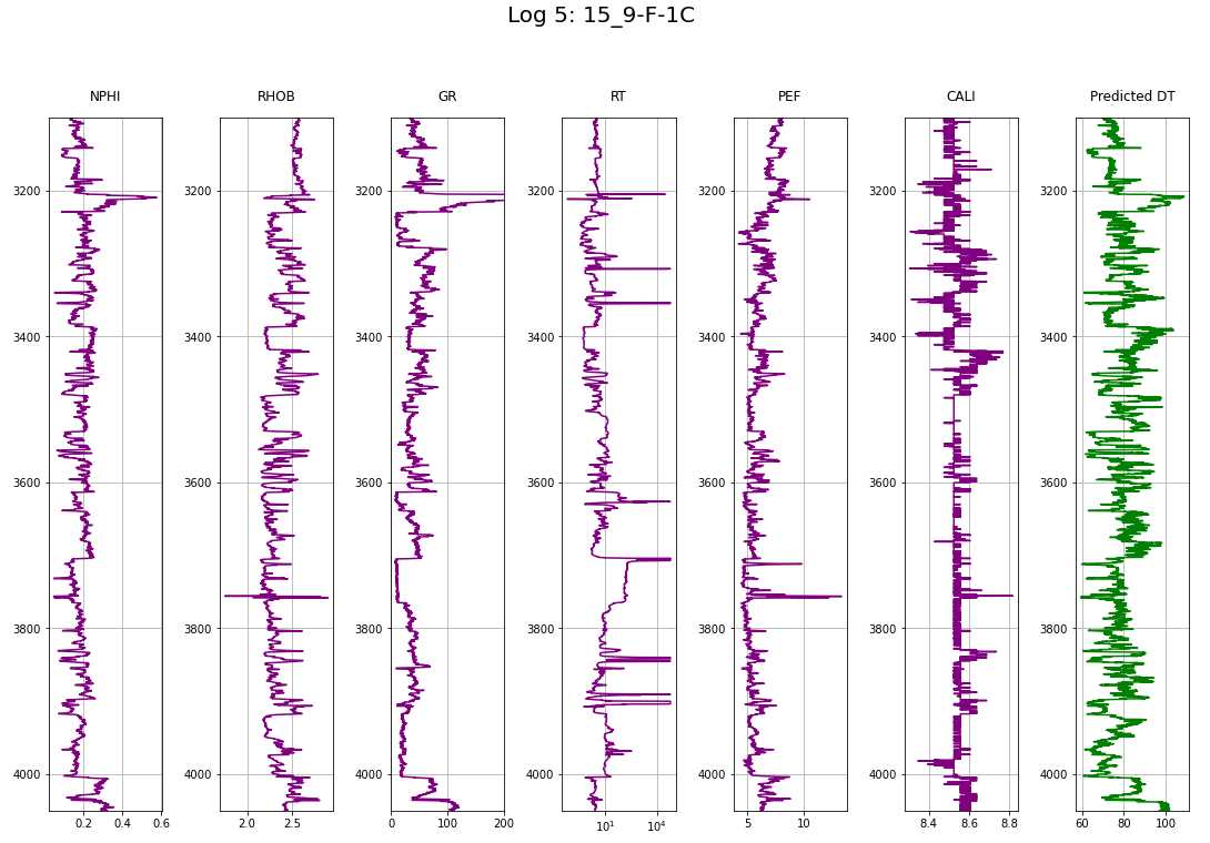
ADV SQL QRIES
CASE
CASE WHEN THEN ELSE END AS. The ELSE and AS are optionalSELECT
m.date,
t.team_long_name AS opponent,
CASE WHEN m.home_goal < m.away_goal THEN 'Barcelona win!'
WHEN m.home_goal > m.away_goal THEN 'Barcelona loss :('
ELSE 'Tie' END AS outcome
FROM matches_spain AS m
LEFT JOIN teams_spain AS t
ON m.hometeam_id = t.team_api_id
WHERE m.awayteam_id = 8634;
CASE and aggregate function (SUM)
SELECT
	c.name AS country,
	SUM(CASE WHEN m.season = '2012/2013' AND m.home_goal > m.away_goal
			 THEN 1 ELSE 0 END) AS matches_2012_2013,

	SUM(CASE WHEN m.season = '2013/2014' AND m.home_goal > m.away_goal
			 THEN 1 ELSE 0 END) AS matches_2013_2014,

	SUM(CASE WHEN m.season = '2014/2015' AND m.home_goal > m.away_goal
			 THEN 1 ELSE 0 END) AS matches_2014_2015
FROM country AS c
LEFT JOIN match AS m
ON c.id = m.country_id
GROUP BY country;
Percentages with AVG and CASE
AVG and CASE (for 1,0 assignment) functions.SELECT
c.name AS country,
ROUND(AVG(CASE WHEN m.season='2013/2014' AND m.home_goal = m.away_goal THEN 1
WHEN m.season='2013/2014' AND m.home_goal != m.away_goal THEN 0
END),2) AS pct_ties_2013_2014,
ROUND(AVG(CASE WHEN m.season='2014/2015' AND m.home_goal = m.away_goal THEN 1
WHEN m.season='2014/2015' AND m.home_goal != m.away_goal THEN 0
END),2) AS pct_ties_2014_2015
FROM country AS c
LEFT JOIN matches AS m
ON c.id = m.country_id
GROUP BY country;
TRY queries and CATCH errors
BEGIN TRY
	ALTER TABLE products
		ADD CONSTRAINT CHK_Stock CHECK (stock >= 0);
END TRY

BEGIN CATCH
	SELECT 'There was an error adding the constraing!';
END CATCH
Nested TRY/CATCH
BEGIN TRY
	INSERT INTO bikes (make, model, year, size)
		VALUES ('Nukeproof', 'Grizzlybear', '2021', 'S');
END TRY

BEGIN CATCH
	SELECT 'An error occurred inserting the bike!';
    BEGIN TRY
    	INSERT INTO errors
        	VALUES ('Error inserting a bike');
        SELECT 'Error inserted correctly!';
	END TRY

    BEGIN CATCH
    	SELECT 'An error occurred inserting the error!';
    END CATCH
END CATCH
CATCH Error Details
BEGIN TRY
	INSERT INTO bikes (make, model, year, size)
		VALUES ('Nukeproof', 'Grizzlybear', '2021', 'S');
END TRY

BEGIN CATCH
	SELECT 'An error occurred inserting the product!';
    BEGIN TRY
    	INSERT INTO errors
        	VALUES ('Error inserting a product');
    END TRY

    BEGIN CATCH
    	SELECT  ERROR_NUMBER() AS number,
        	ERROR_SEVERITY() AS severity_level,
        	ERROR_STATE() AS state,
        	ERROR_LINE() AS line,
        	ERROR_MESSAGE() AS message;
    END CATCH
END CATCH
Custom Errors, RAISERROR
RAISERROR ( { msg_str | msg_id | @local_variable_message },
    severity,
    state,
    [ argument [ ,...n ] ] )
    [ WITH option [ ,...n ] ]
@product_id = 56747

BEGIN TRY
IF NOT EXISTS (SELECT * FROM products WHERE product_id = @product_id)
	RAISERROR('No product with id %d.', 11, 1, @product_id);
ELSE
	SELECT * FROM products WHERE product_id = @product_id;
END TRY

BEGIN CATCH
    SELECT  ERROR_NUMBER() AS number,
        ERROR_SEVERITY() AS severity_level,
        ERROR_STATE() AS state,
        ERROR_LINE() AS line,
        ERROR_MESSAGE() AS message;
END CATCH
Subqueries
Subqueries in WHERE clause
SELECT
	team_long_name,
	team_short_name
FROM team
WHERE team_api_id IN
	(SELECT hometeam_id
	 FROM match
	 WHERE home_goal >= 8);
Subqueries in FROM
SELECT
	country,
	date,
	home_goal,
	away_goal
FROM
	(SELECT c.name AS country,
			m.date,
			m.home_goal,
			m.away_goal,
			(m.home_goal + m.away_goal) AS total_goals
	FROM match AS m
	LEFT JOIN country AS c
	ON m.country_id = c.id) AS subq
WHERE total_goals >= 10;
Subqueries in SELECT
SELECT statements generate a single value!SELECT
l.name AS league,
ROUND(AVG(m.home_goal + m.away_goal), 2) AS avg_goals
(SELECT ROUND(AVG(home_goal + away_goal), 2)
FROM match
WHERE season = '2013/2014') AS overall_avg
FROM league AS l
LEFT JOIN match AS m
ON l.country_id = m.country_id
WHERE season = '2013/2014'
GROUP BY league;
Correlated Subqueries
WHERE clause filters for entries with total goals higher than three times the average.SELECT
main.country_id,
date,
main.home_goal,
main.away_goal
FROM match AS main
WHERE
(home_goal + away_goal) >
(SELECT AVG((sub.home_goal + sub.away_goal) * 3)
FROM match AS sub
WHERE main.country_id = sub.country_id);
Nested Subqueries in FROM
SELECT
	c.name AS country,
	AVG(outer_s.matches) AS avg_seasonal_high_scores
FROM country AS c
LEFT JOIN (
		SELECT country_id, season,
			COUNT(id) AS matches
		FROM (
			SELECT country_id, season, id
			FROM match
			WHERE home_goal >= 5 OR away_goal >= 5) AS inner_s
		GROUP BY country_id, season) AS outer_s
ON c.id = outer_s.country_id
GROUP BY country;
Common Table Expressions (CTE)
WITH cte AS (SELECT…..)WITH home AS (
SELECT m.id,
m.date,
t.team_long_name AS hometeam,
m.home_goal
FROM match AS m
LEFT JOIN team AS t
ON m.hometeam_id = t.team_api_id),
away AS (
SELECT m.id,
m.date,
t.team_long_name AS awayteam,
m.away_goal
FROM match AS m
LEFT JOIN team AS t
ON m.awayteam_id = t.team_api_id)
SELECT
home.date,
home.hometeam,
away.awayteam,
home.home_goal,
away.away_goal
FROM home
INNER JOIN away
ON home.id = away.id;
Window Functions - They all use OVER()
OVER() clause allows you to pass an aggregate function down a data set, similar to subqueries in SELECT, but run faster.OVER() generates column with an aggregate of the complete column and the same value in each row.SELECT
m.id,
c.name AS country,
m.season,
m.home_goal,
m.away_goal,
AVG(m.home_goal + m.away_goal) OVER() AS overall_avg
FROM match AS m
LEFT JOIN country AS c ON m.country_id = c.id;
OVER(ORDER BY...) calculates the running total/sum up to the current row.SELECT
athlete,
medals,
SUM(medals) OVER(ORDER BY athlete ASC) AS sum_medals
FROM athlete_medals
ORDER BY athlete ASC;
RANK()
SELECT
	l.name AS league,
	AVG(m.home_goal + m.away_goal) AS avg_goals,
	RANK() OVER(ORDER BY AVG(m.home_goal + m.away_goal) DESC) AS league_rank
FROM league AS l
LEFT JOIN match AS m
ON l.id = m.country_id
WHERE m.season = '2011/2012'
GROUP BY l.name
ORDER BY league_rank;
SELECT
  athlete,
  medals,
  RANK() OVER (ORDER BY medals DESC) AS Rank_N
FROM Athlete_Medals
ORDER BY Medals DESC;
DENSE_RANK()
SELECT
  country,
  athlete,
  DENSE_RANK() OVER (PARTITION BY country ORDER BY medals DESC) AS rank_n
FROM athlete_medals
ORDER BY country ASC, rank_n ASC;
Giving rows a number with ROW_NUMBER()
ROW_NUMBER().SELECT
*,
ROW_NUMBER() OVER() AS Row_N
FROM Summer_Medals
ORDER BY Row_N AS
ORDER BY inside the OVER() clause takes precedence over outer ORDER BY. The following queries only calls distinct years and does not requrie a subquery.SELECT
Year,
ROW_NUMBER() OVER(ORDER BY Year ASC) AS Row_N
FROM (
SELECT DISTINCT Year
FROM Summer_Medals
) AS Yea
Framing for sliding windows using RANGE BETWEEN…AND or ROWS BETWEEN…AND
UNBOUNDED, n PRECEDING, n FOLLOWING, and CURRENT ROWRANGE vs. ROW: RANGE() treats duplicates in OVER(ORDER BY...) as a single entity, which is a special case. ROWS behaves normally.Medals Rows Running Total Range Running Total 10 10 10 50 60 110 50 110 110 60 170 230 60 230 230 70 300 300 SELECT
date,
home_goal,
away_goal,
SUM(home_goal) OVER(ORDER BY date
ROWS BETWEEN UNBOUNDED PRECEDING AND CURRENT ROW) AS running_total,
AVG(home_goal) OVER(ORDER BY date
ROWS BETWEEN UNBOUNDED PRECEDING AND CURRENT ROW) AS running_avg
FROM match
WHERE
hometeam_id = 9908
AND season = '2011/2012';
SELECT
	date,
	home_goal,
	away_goal,
	SUM(home_goal) OVER(ORDER BY date DESC
		ROWS BETWEEN CURRENT ROW AND UNBOUNDED FOLLOWING) AS running_total,
	AVG(home_goal) OVER(ORDER BY date DESC
		ROWS BETWEEN CURRENT ROW AND UNBOUNDED FOLLOWING) AS running_avg
FROM match
WHERE
	awayteam_id = 9908
    AND season = '2011/2012';
SELECT
	year,
	medals,
	AVG(medals) OVER(ORDER BY year ASC
		ROWS BETWEEN 2 PRECEDING AND CURRENT ROW) AS medals_ma
FROM russian_medals
ORDER BY year ASC;
Fetching relative rows: LAG() and LEAD()
LAG(column, n) function fetches a single value from BEFORE (above) the current row (given vertical lag distance) for creating a new column.SELECT
Year, Champion,
LAG(Champion) OVER(ORDER BY year ASC) AS Last_Champion
FROM weightlifting_gold
ORDER BY year ASC;
LEAD(column, n) function fetches a single value from AFTER (below) the current row (given vertical lag distance) for creating a new column.SELECT
year,
athlete,
LEAD(athlete, 3) OVER (ORDER BY year ASC) AS future_champion
FROM discus_medalists
ORDER BY year ASC;
Fetching absolute rows: FIRST_VALUE() and LAST_VALUE()
FIRST_VALUE(column) and LAST_VALUE(column)SELECT
athlete,
FIRST_VALUE(athlete) OVER(ORDER BY athlete ASC) AS First_Athlete
FROM all_male_medalists;
RANGE BETWEEN UNBOUNDED PRECEDING AND UNBOUNDED FOLLOWING.SELECT
year,
city,
LAST_VALUE(city) OVER(ORDER BY year ASC
RANGE BETWEEN
UNBOUNDED PRECEDING AND
UNBOUNDED FOLLOWING
) AS last_city
FROM hosts
ORDER BY Year ASC;
PARTITION BY subdivides processing ranges in a column
ROW_NUMBER or LAG() functions.LAG() function determining gold winners of ‘male’ spilling into ‘females’. In that case, a null value will be displayed.SELECT
gender,
year,
country AS champion,
LAG(country,1) OVER(PARTITION BY gender ORDER BY year ASC) AS last_champion
FROM athletics_gold
ORDER BY gender ASC, year ASC;
SELECT
	gender,
	year,
	event,
	country AS champion,
	LAG(country,1) OVER (PARTITION BY gender, event ORDER BY year ASC) AS last_champion
FROM athletics_gold
ORDER BY event ASC, gender ASC, year ASC;
Paging with NTILE()- subdivide a table into equal-length pages
NTILE(num_pages) OVER(ORDER BY column) AS new_column divides the table into num_pages depending on how the values in the given column. The new column contains the number of which page they were assigned. These pages are practically quantiles on which statistical analysis can be performed.SELECT
athlete,
medals,
NTILE(3) OVER(ORDER BY medals DESC) AS third
FROM athlete_medals
ORDER BY medals DESC, athlete ASC;
WITH thirds AS (
	SELECT
		athlete,
		medals,
		NTILE(3) OVER(ORDER BY medals DESC) AS third
	FROM athlete_medals)

SELECT
	third,
	AVG(medals) AS avg_medals
FROM thirds
GROUP BY third
ORDER BY third ASC;
Pivoting with the CROSSTAB() Extension
CROSSTAB requires the tablefunc extension that needs to be created befor qerrying.SELECT * FROM CROSSTAB($$....) AS ct (column COLTYPE,...) function and the new pivoted column names defined.CREATE EXTENSION IF NOT EXISTS tablefunc;
SELECT * FROM CROSSTAB($$
SELECT
gender,
year,
country
FROM summer_medals
WHERE
year IN (2008, 2012)
AND medal = 'gold'
AND event = 'pole vault'
ORDER BY gender ASC, year ASC;
$$) AS ct (gender VARCHAR,
"2008" VARCHAR,
"2012" VARCHAR)
ORDER BY gender ASC;
gender year country Men 2008 AUS Men 2012 FRA Women 2008 RUS Women 2012 USA gender 2008 2012 Men AUS FRA Women RUS USA Group total rows with GROUP BY ROLLUP() and CUBE()
Null entries in the rows signifies the total rows.ROLLUP(gender) clause.SELECT
country,
gender,
COUNT(*) AS gold_awards
FROM summer_medals
WHERE
year = 2004
AND medal = 'Gold'
AND country IN ('DEN', 'NOR', 'SWE')
GROUP BY country, ROLLUP(gender)
ORDER BY country ASC, gender ASC;
CUBE(). Note: all columns have to go into the CUBE() or it will fail.SELECT
gender,
medal,
COUNT(*) AS awards
FROM Summer_Medals
WHERE
year = 2012
AND country = 'RUS'
GROUP BY CUBE(gender, medal)
ORDER BY gender ASC, medal ASC;
Fill Null values with COALESCE()
ROLLUP(), CUBE(), pivoting, first/last row of LAG(), LEAD().SELECT section of query: COALESCE(column, 'null filler string') AS column.SELECT
COALESCE(country, 'all countries') AS country,
COALESCE(gender, 'all genders') AS gender,
COUNT(*) AS awards
FROM summer_medals
WHERE
year = 2004
AND medal = 'gold'
AND country IN ('DEN', 'NOR', 'SWE')
GROUP BY ROLLUP(country, cender)
ORDER BY country ASC, gender ASC;
String Manipulation
Compress a Column into a single String with STRING_AGG()
SELECT statemtt like as such: STRING_AGG(column, 'separator')SELECT
STRING_AGG(country, ', ')
FROM country_ranks
WHERE rank_col <= 3;
Country Rank USA 1 RUS 2 AUS 3 … … Concatenating Multiple Columns with || and CONCAT()
SELECT
	first_name || ' ' || last_name AS full_name
FROM
	film;
SELECT
	customerID || ': ' || first_name || ' ' || last_name AS full_name;
CONCAT()SELECT
CONCAT(first_name,' ', last_name) AS full_name
FROM
film;
Changing Case with UPPER(), LOWER(), INITCAP()
SELECT
	UPPER(email)
FROM customer;
SELECT
	LOWER(email)
FROM customer;
SELECT
	INITCAP(title)
FROM film;
Replace Characters with REPLACE()
SELECT
	REPLACE(email, 'hedgeAThog.com', '[email protected]') AS email
FROM customer;
Trim Characters with TRIM(), LTRIM(), RTRIM()
TRIM([leading | trailing | both][characters] from string)space chars is be removed by default.space char is the default.SELECT
TRIM(),
LTRIM(' [email protected] '),
RTRIM(' [email protected] ')
Pad Characters with PAD(), LPAD(), RPAD()
LPAD(input_string, length_after_pad, lpad_string) Note that if the input string is shorter than the padded length, then no padding string will be inserted! If no padding string passed, is entered, then space char is the default.SELECT
LPAD('[email protected]', 20, '#'),
RPAD('[email protected]', 17, '$')
Reverse char order with REVERSE()
SELECT
	email,
	REVERSE(email)
FROM customer;
Character Count with CHAR_LENGTH() or LENGTH()
SELECT
	title,
	CHAR_LENGTH(title)
	LENGTH(title)
FROM film;
Find Char Position with STRPOS() or POSITION()
SELECT
	email,
	STRPOS(email, '@'),
	POSITION('@' IN email)
FROM customer;
Clip Strings from the Ends with LEFT(), RIGHT(), and SUBSTRING()
SELECT
	RIGHT(column_name, 50),
	LEFT(column_name, 10)
FROM customer;
SELECT
	SUBSTRING(column_name, 10, 50),
	SUBSTR(colum_name, 10, 50)
FROM customer;
SELECT
	SUBSTRING(email FROM 0 FOR POSITION('@' IN email)), -- name part of address up to @
	SUBSTRING(email FROM POSITION('@' IN email)+1 FOR CHAR_LENGTH(email)) -- provider part of address starting after @
FROM customer;
SELECT
	LEFT(description, 50 - POSITION(' ' IN REVERSE(LEFT(description, 50)) -- Subtract the position of the first whitespace character
FROM film;
Data Types
Casting Data Types
column :: data-typeSELECT
NOW():: timestamp;
CAST(column AS data-type) function.SELECT
CAST(NOW() AS timestamp);
Creating Data Types (PostgreSQL)
CREATE
	TYPE dayofweek as ENUM(
		'Monday',
		'Tuesday',
		'Wednesday',
		'Thursday',
		'Friday',
		'Saturday',
		'Sunday'
		);
Getting Information about Data Types (PostgreSQL)
SELECT
	typname,
	typcategory
FROM pg_type
WHERE typname = 'dayofweek';
User-Defined Functions (PostgreSQL)
CREATE.CREATE FUNCTION squared (i integer) RETURNS integer AS $$
BEGIN
RETURN i*i;
END;
$$ language plpgsql; --define language
SELECT
squared(10);
Text Search and NLP (PostgreSQL)
Full-Text Search (PostgreSQL)
WHERE column LIKE '%mystring%' with wildcards (%,_) etc. capabilities.SELECT
title,
description
FROM film
WHERE to_tsvector(title) @@ to_tsquery('elf');
Compare Two Strings (PostgreSQL)
SELECT
	levenshtein('hugo', 'hagolm');
similarity('hugo', 'hagolm');
Drop Duplicate Rows (based on Specific Columns)
WITH cte AS (
    SELECT *,
        ROW_NUMBER() OVER (
            PARTITION BY
                col_1,
                col_2,
                col_3
			ORDER BY
                col_1,
                col_2,
                col_3
        ) row_num
    FROM orders_table
)
SELECT *
FROM cte
WHERE row_num = 1;
id sales worker_firstname worker_lastname registration_date row_num 000000119 13 Johnny Smith 2014-01-31 1 000000127 14 Brian Merkel 2014-02-28 1 000000120 29 Karin Harris 2014-01-31 1 000000128 16 Carol Schulze 2014-02-28 1 Time Manipulation
NOW() and CURRENT_TIMESTAMP() fetch time (millisecond precision) with timezone! However, CURRENT_TIMESTAMP(2) can be passed an argument for roundeding to digits. If the timezone is not required, then these two functions can be cast to timestamp data-type.CURRENT_DATE only fetches the date portion of the CURRENT_TIMESTAMP()CURRENT_TIME() only fetches the time portion (with timezone) of the CURRENT_TIMESTAMP(). Can be passed rounding parameter.Intervals and Time Differences
INTERVAL function. The INTERVAL add 3 days to the rental date so we can compare if the return date was in time.SELECT
rental_date,
return_date,
rental_date + INTERVAL '+ `+3 days' AS expected_return_date
FROM rental;
SELECT
	title,
	INTERVAL '1' day * f.rental_duration AS rental_duration,
	return_date - rental_date AS days_rented
FROM film
WHERE return_date IS NOT NULL
AGE() function calculates an INTERVAL between a given timestamp/date and NOW if ONE parameter given. If TWO parameters are given, then the interval between those.SELECT
AGE(rental_date)
FROM rental;
Extracting from Timestamps
EXTRACT(field FROM source) and DATE_PART('field',source), which produce interchangeable results.Field (long) Field (short) Description year y Year quarter Quarter month Month day d Day of Month dow Day of Week week w Week hour h hour minute m Minute second s Second millisecond ms Millisecond SELECT
EXTRACT(quarter FROM TIMESTAMP '2009-02-12 05:18:00') AS quarter;
SELECT
	DATE_PART('quarter', TIMESTAMP '2009-02-12 05:18:00') AS quarter;
SELECT
	EXTRACT(dow FROM rental_date) AS dayofweek,
	COUNT(*) as rentals
FROM rental
GROUP BY 1; -- column called by positional index instead of names
SELECT
	EXTRACT(quarter FROM payment_date) AS quarter,
	EXTRACT(year FROM payment_date) AS year,
	SUM(amount) AS total_payments
FROM payment
GROUP BY 1, 2;
SELECT
	EXTRACT(dow FROM r.rental_date) AS dayofweek,
	AGE(return_date, rental_date) AS rental_days
FROM rental AS r
WHERE rental_date
	BETWEEN CAST('2005-05-01' AS TIMESTAMP)
	AND CAST('2005-05-01' AS TIMESTAMP) + INTERVAL '90 day';
Truncating Timestamps
DATE_TRUNC() function will truncate a timmestamp or interval data types from fine detail (e.g., minutes) to low detail (e.g., year). This means the timestamp’s length remains the same but set to the lowest logical value (01 for days/months, 00 for hours/minutes/seconds).SELECT
DATE_TRUNC('year', TIMESTAMP '2009-02-12 05:18:00';
SELECT
	DATE_TRUNC('month', TIMESTAMP '2009-02-12 05:18:00';
SELECT
	DATE_TRUNC('day', rental_date) AS rental_day,
	COUNT(*) AS rentals
FROM rental
GROUP BY 1;
Transactions (MS SQL SERVER)
With TRY/CATCH
BEGIN TRY
	BEGIN TRAN;
		UPDATE accounts SET current_balance = current_balance - 100 WHERE account_id = 4451;
		INSERT INTO transactions VALUES (4451, -100, GETDATE());

		UPDATE accounts SET current_balance = current_balance + 100 WHERE account_id = 6743;
		INSERT INTO transactions VALUES (4451, 100, GETDATE());
	COMMIT TRAN;
END TRY

BEGIN CATCH
	SELECT 'Rolling back the transaction';
	ROLLBACK TRAN;
END CATCH
With XACT_ABORT
SET XACT_ABORT ON;

BEGIN TRAN;
	UPDATE accounts set current_balance = current_balance - current_balance * 0.01 / 100
		WHERE current_balance > 5000000;
	IF @@ROWCOUNT <= 10
		THROW 55000, 'Not enough wealthy customers!', 1;
	ELSE
		COMMIT TRAN;
Special Case: Accessing ARRAYS
SELECT
	email[1][1] AS type,			-- select from first address the first element (address type/description)
	email[1][2] AS address,			-- select from first address the second element (email address)
	test_scores[1]				    -- select only first element of the array
FROM funky_table
WHERE email[1][1] = "work";			-- only search in in array element 1 and sub-element 1
ANY or @> operators. Results are equivalent.SELECT
email[2][1] AS type, -- select from second address the first element (address type/description)
email[2][2] AS address, -- select from second address the second element (email address)
test_scores[1] -- select only first element of the array
FROM funky_table
WHERE 'home' = ANY (email) -- select where the column `email` contains an array element named 'home' in any array position)
SELECT
  email[2][1] AS type,
  email[2][2] AS address
  test_scores[1]
FROM funky_table
WHERE email @> ARRAY['home'];
SQL query in Python Pandas
import sqlalchemy

connection_uri = "postgresql://repl:password@localhost:5432/pagila"
db_engine = sqlalchemy.create_engine(connection_uri)

import pandas as pd

df = pd.read_sql("""
SELECT
    first_name,
    last_name
FROM "Customer"
ORDER BY last_name, first_name
""", db_engine)

df.head(3)
first_name last_name 0 Connagh Bailey 1 Brook Bloom 2 Ann Dalton ETL process
import sqlalchemy
import pandas as pd

# custom extraction function
def extract_table_to_pandas(tablename, db_engine):
    query = "SELECT * FROM {}".format(tablename)
    return pd.read_sql(query, db_engine)

connection_uri = "postgresql://repl:password@localhost:5432/pagila"
db_engine = sqlalchemy.create_engine(connection_uri)

extract_table_to_pandas("film", db_engine)
connection_uri = "postgresql://repl:password@localhost:5432/dwh"
db_engine_dwh = sqlalchemy.create_engine(connection_uri)

film_pdf_joined.to_sql("film", db_engine_dwh, schema="store", if_exists="replace")

# check the table in the SQL db
pd.read_sql("SELECT film_id, recommended_film_ids FROM store.film", db_engine_dwh)
Table Management
Create Table
CREATE TABLE funky_table (
	column_1 text,
	column_2 integer,
	column_3 scores[],
	employee_id integer,
	email text[][]
	);
Insert Values into Columns
INERT INTO funnky_table
	(column_1, column_2) VALUES ('string for column_1', 12);
INSERT INTO funky_table
	VALUES ("Prickly Hedgehog",
		2,
		{99,83,18,811}, -- standard array with four elements
		2224,
		{\{"work", "[email protected]"},{"home", "[email protected]"}}  -- nested array (remove escape char \)
		);
System Database Information Gathering
SELECT *
FROM
	information_schema.tables
WHERE
	table_schema = 'public';
SELECT *
FROM
	information_schema.columns
WHERE
	table_name = 'actor';
table_catalog table_schema table_name column_name ordinal_position column_default is_nullable data_type character_maximum_length ….. and so on.Extension Management (PostgreSQL)
Show Extensions
SELECT
	name
FROM pg_available_extensions;
SELECT
	extname
FROM pg_extension;
Install/Import Extensions
CREATE EXTENSION IF NOT EXISTS fuzzystrmatch;
SELECT
	extname
FROM pg_extension;
The New Business of AI (and How It’s Different From Traditional Software) - a16z

Preface
Introduction
Software + Services = AI?
Software Company
Service Company
AI Company
Gross Margins, Part 1: Cloud costs can be massive for AI
Gross Margins, Part 2: Many AI applications rely on “humans in the loop”
Scaling AI systems can be rockier - AI lives in the long tail
The how to defend AI businesses has to be figured out
Building, scaling, and defending great AI companies – practical advice for founders
Summary
Taming the Tail - Adventures in Improving AI Economics - a16z
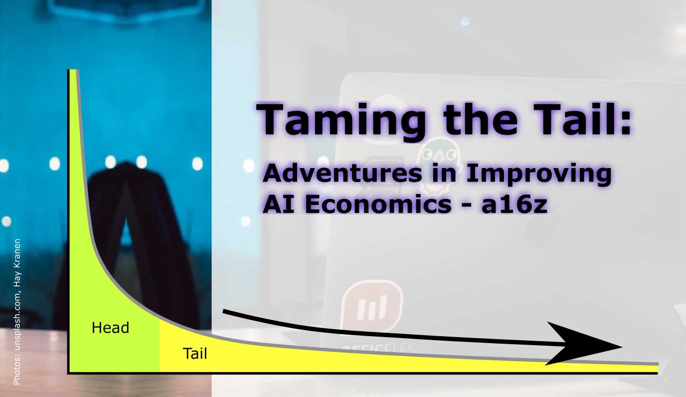
Preface
Introduction
Part I: Understanding the problem to be solved
Building vs. experimenting (or, software vs. AI)
The long tail and machine learning
Impact on the economics of AI
Part II: Building Better AI Systems
Toward a Solution
Easy mode: Bounded problems
Harder: Global long tail problems
Really hard: Local long tail problems
Table stakes: Operations
Summary
My Machine Learning Model Is Perfect

Code that needs refactoring
Breakout: Who has the smelliest code?
What does Machine Learning smell like?
PhD Résumé and CoverLetter Template

Introduction
How to
Preview
Résumé


CoverLetter
Physicists Dissecting "Interstellar"

Accurate Science Fiction?
Bonus
Reading in 2020

Introduction
R.S. Sutton and A.G. Barto: “Reinforcement Learning: An Introduction”

G.R.R Martin: “A Dance with Dragons”

P. Domingos: “The Master Algorithm”
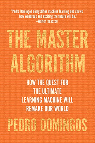
C. Thompson: “Coders”

S. Pinker: “The Sense of Style”

Fashion MNIST

Introduction

Hands-On
R, the following functions should do the job and load the training and test cases including class labels into the global environment. The code was provided by <href=”https://gist.github.com/brendano/39760” target=”_blank”>Brendan O’Connor</a>:load_mnist <- function() {
load_image_file <- function(filename) {
ret = list()
f = file(filename,'rb')
readBin(f,'integer',n=1,size=4,endian='big')
ret$n = readBin(f,'integer',n=1,size=4,endian='big')
nrow = readBin(f,'integer',n=1,size=4,endian='big')
ncol = readBin(f,'integer',n=1,size=4,endian='big')
x = readBin(f,'integer',n=ret$n*nrow*ncol,size=1,signed=F)
ret$x = matrix(x, ncol=nrow*ncol, byrow=T)
close(f)
ret
}
load_label_file <- function(filename) {
f = file(filename,'rb')
readBin(f,'integer',n=1,size=4,endian='big')
n = readBin(f,'integer',n=1,size=4,endian='big')
y = readBin(f,'integer',n=n,size=1,signed=F)
close(f)
y
}
train <<- load_image_file('train-images-idx3-ubyte')
test <<- load_image_file('t10k-images-idx3-ubyte')
train$y <<- load_label_file('train-labels-idx1-ubyte')
test$y <<- load_label_file('t10k-labels-idx1-ubyte')
}
show_digit <- function(arr784, col=gray(12:1/12), ...) {
image(matrix(arr784, nrow=28)[,28:1], col=col, ...)
}
library(reshape2)
library(ggplot2)


showExamples <- function(nExamplesClass = 10, randomize = F) {
  classes <- sort(unique(train$y)) # a vector of all classes
  nClasses <- length(classes) # Number of classes
  iExamples <- as.matrix(sapply(classes,
                                function(i) {
                                  iLab <- which(train$y == i)
                                  sample(x = iLab, size = nExamplesClass, replace = F)
                                }))
  if(randomize) {
    iExamples <- matrix(sample(x = iExamples, size = length(iExamples), replace = F),
                  nrow = dim(iExamples)[1])
  }

  data <- array(train$x[iExamples, ], dim = c(nExamplesClass * nClasses, 28, 28))
  plotData <- melt(data, varnames = c("image", "x", "y"), value.name = "pixel")
  nrows <- if(randomize) round(sqrt(nExamplesClass * nClasses)) else 10
  p <- ggplot(plotData, aes(x = x, y = y, fill = pixel)) +
    geom_tile() +
    scale_y_reverse() +
    facet_wrap(~ image, nrow = nrows) +
    theme_bw()+
    theme(
      panel.spacing = unit(0, "lines"),
      axis.text = element_blank(),
      axis.ticks = element_blank(),
      strip.background = element_blank(),
      strip.text.x = element_blank(),
      panel.grid.major = element_blank(),
      panel.grid.minor = element_blank(),
      legend.position   = "none",
      axis.title.x = element_blank(),
      axis.text.x = element_blank(),
      axis.ticks.x = element_blank(),
      axis.title.y = element_blank(),
      axis.text.y = element_blank(),
      axis.ticks.y = element_blank()
    ) + scale_fill_gradient(low = "black", high = "white")

  plot(p)
}
showExamples(20, T) we can plot a 20x20 matrix with 400 random images: 

Google ML introducing Fashion MNIST
A Peek Behind the ML Curtain

estimated with the rigor of our choosing. In statistics, this concept is formalized in estimation theory. This article shows how this can be applied to ML and how we quantify the quality of a model. Since ML models can generally not be perfect for complex problems, it is useful to try to describe how good they are.Estimator Properties
Bias
Variance

Bias-Variance Tradeoff

Gradient Descent
Full-Batch Gradient Descent
Stochastic Gradient Descent
Mini-Batch Gradient Descent

Conclusion
gem "kramdown-math-katex"Pagination